The heart is one of the most vital organs in our body, with its primary function being to move blood throughout the body. Despite this, there are several health issues that it might cause. Problems with the heart and blood vessels are known as cardiovascular diseases (CVD). The most common killer in the modern world is cardiovascular disease, which manifests mostly as heart attacks and strokes. About 32% of all fatalities occur because of cardiovascular disease, which accounts for 17.9 million deaths annually [1]. Four out of five deaths caused by cardiovascular disease occur because of heart attacks or strokes [2]. Because of its size and importance, the heart requires special attention. Predicting cardiac problems is crucial, necessitating comparative study in this area, as most diseases have some connection to the heart. More effective disease prediction algorithms are required because most people die because their illnesses are only discovered at a late stage because of inaccurate medical instruments [3]. There are a lot of risk factors for heart disease, such as being overweight, having high cholesterol, smoking, not eating well, having diabetes, and having irregular heart rhythms [4]. Problems with the heart's melody, valves, tissues, infections, blood arteries, or congenital abnormalities are all examples of heart diseases. Globally, coronary disease (CHD) ranks highest among the many forms of heart illness (HD) that account for many fatalities. Several symptoms, such as vertigo, fainting, irregular heartbeat, difficulty breathing, etc., can be noted due to these various kinds. Meditation, regular exercise, a good diet, and other lifestyle changes can greatly reduce the risk of cardiovascular disease, which can be fatal if left untreated. More and more, doctors are turning to artificial intelligence (AI) to help diagnose serious illnesses like cancer, diabetes, and heart disease.
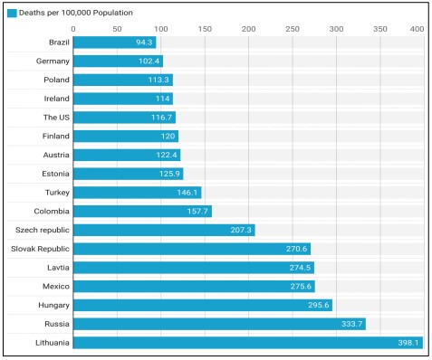
Figure 1. Ischemic Heart Disease Deaths per 100,000 Population in OECD Countries [5].
Artificial intelligence (AI) refers to a wide range of techniques, including analytical algorithms that learn from data iteratively, enabling computers to find secret knowledge without being told specifically where to look. In cases when conventional statistical approaches fail, this set of procedures may integrate and make sense of complex biological and healthcare data using terms like deep learning, artificial intelligence, cognitive learning, and reinforcement learning. [6]. Researchers are striving to develop an effective methodology for the early detection of a cardiovascular ailment because current approaches to heart disease diagnostics are ineffective in early detection for several reasons, such as accuracy and execution time. Without access to modern diagnostic tools and trained medical professionals, heart disease is notoriously difficult to detect and treat [7]. Figure 1 shows that ischemic heart disease death rates vary significantly between nations. That's why it's critical to implement targeted interventions and improve healthcare methods in those countries with the highest rates to lower these avoidable deaths.
Our research explores the classification of heart disease using a comprehensive dataset that encompasses various clinical and demographic attributes. We extracted the Heart Disease Classification dataset from Kaggle [8]. Data pre-processing included various stages such as normalization, one-hot encoding, and outlier detection and removal. The input variables for modeling were preprocessed through Principal Component Analysis (PCA). We perform model training and assessment through algorithm comparison, where we considered Logistic Regression, KNN, Naive Bayes, SVM, Decision Tree, and Random Forest when with or without the use of PCA. Since it is aimed to compare the models comprehensively, several comparisons were made to assess the performance before and after the elimination of outliers together with that of noise. Lastly, it is the purpose of this research to create a solid comprehension of the heart disease classification and devise realistic ideas helpful for clinical decision-makers and the field of health care.
As follows, the manuscript consists of the following sections: Section II provides an overview of previous studies as a background and literature review of our study. Section III is divided into two subsections: the first covers the dataset, while the second outlines the methodology used in our experiments. In Section IV, we present and analyze the results of our models. Section V is about discussion. Finally, Section VI concludes the paper with a summary of our findings and suggestions for future research.
Novelty and Objectives of Study
• Cross-analytics assessment of Random Forest, SVM, and Logistic Regression algorithms for accurate heart disease diagnosis using sophisticated noise reduction and outlier elimination methodologies which are lacking in the earlier literature review.
• Increasing accuracy and AUC (Area Under the Curve) of heart disease classification than previous studies by improving the selection of features, using data preprocessing techniques such as noise reduction process and outlier removal, and tuning the model parameters.
• Offering a comprehensive analysis of the performance of identified models across different measures; revealing how much usefulness noise reduction and outlier elimination bring about in improving the performances of classification models in heart disease-related problems.
The purpose of this study is to select the best machine learning model for the prediction of heart disease and its performance should be better when compared to the works done earlier.
Literature Review
Researchers have found shared features in the datasets they've worked with in various studies and tests with heart disease. A list of prior research indicating the datasets utilized and assembled is provided below. For this investigation, we will be using this integrated dataset. Given in [9] The authors of this work offer a method for detecting heart illness by using selecting and categorizing features algorithms. Feature selection methods are utilized in feature engineering, with the Sequential Backwards Selecting Algorithm (SBS FS) being the algorithm of choice. For this model's evaluation, we turned to the Cleveland coronary artery disease dataset. We used 70% of the dataset for training and 30% for validation. The performance of the proposed system has been examined using evaluation measures. Our evaluation focuses on the classier K-Nearest Neighbor (K-NN) performance on both full and partial feature sets. The proposed method achieved a 90% success rate in making predictions.
Article authors [10] used a dataset on cardiovascular disease to test and implement six ML models: LR, AB, KNN, CART, XGB, and RF. The ROC-AUC scores for the RF model are 0.917 and 84.8%, proving that their results were accurate. A method for the potential future of heart disease (HD) using ML models such as RF, NB, SVM, Hoeffding DT, and Logistic Models Tree (LMT) was laid out by the authors in [11]. Incorporating the CD allowed us to train the models. Accuracy rates of 95.08% for RF and 93.44% for Gaussian-NB demonstrate their strong performance. According to [12], cardiovascular disease is a major global health concern and a major killer worldwide. But because these diseases are complex and expensive, it is hard for doctors to forecast them. In order to help medical professionals with cardiac disease prediction, diagnosis, and decision-making, the researchers in this study suggested a clinical support system.
In this research, various machine learning algorithms were utilized to forecast the occurrence of heart failure by analyzing risk factor data extracted from patient records. These algorithms included Naïve Bayes, KNN, SVM, RF, and DT. Experiments on the HD UCI data set have shown mixed results, with the greatest results coming from NB when combined with cross-validations (82.17% accuracy) and split-test training (84.28% accuracy). Classifiers based on these are developed and a comparison study is conducted in order to produce a dependable prediction of cardiac illness [13]. The Cleveland Heart Failure Data set is utilized to extensively evaluate the five ML algorithms that have been built. Logical regression, Naive Bayes, Support Vector Machine, Random Forest, and K-Nearest Neighbor are the classifiers in question. Following pre-processing, divide the dataset in half lengthwise, with half going into training and half into testing. Identifying cardiac illness is possible with the help of numerous popular classification systems. The effectiveness of each model in detecting heart illness is demonstrated through a comparative analysis of machine-learning approaches. Hyperparameters allow for the tuning of the receiver operating characteristics of binary classifiers trained on pre-processed data.
With LR achieving the best accuracy of 0.93, the authors of [14] laid out the KNN model as the foundational way for predicting cardiovascular illnesses using a feature selection-based methodology. As part of this effort, we used the well-known CD dataset. Although KNN was effective on its own, the authors further improved the method's accuracy by using standardization, feature selection, and cross-validation. Out of 75 overall qualities, 14 were deemed relevant for the procedure. The mean Accuracy, which is 89.23%, was measured using the ten-fold CV. For forecasting cardiac illnesses, the authors in [15] made use of an open-source dataset. To train the dataset, they used five distinct ML algorithms: KNN, DT, RF, NB, and SVM. A few metrics were employed to determine the model's performance efficacy, including Acc, specificity, and Re. With an accuracy of 85%, KNN outperformed the others. For CVD classification, the authors of [16] utilized five ML algorithms: SVM, NB, KNN, DT, and LR. The prediction models were constructed using an open-source dataset that had 77,000 cases. A variety of performance criteria were used to evaluate the models. With accuracy scores of 72.66% and 72.36%, respectively, LR and SVM were noted as effective algorithms for identifying anomalies related to CVD.
To anticipate CVD early and affordably, the article [17] investigated the use of ML models. An assortment of strategies, including NB, DT, RF, KNN, SVM, and LR, were utilized for the purpose of CVD prediction. After converting the CD to acumen by parameter measurement, the model's prediction was completed with the RF achieving the greatest Acc of 83.52%. The scientists employed various supervised models based on machines to forecast cardiac illnesses [18]. In all, there are 303 instances and 14 attributes in the dataset that were utilized for their study. Incorporating algorithms such as LR, KNN, and SVM, the effectiveness of these models was evaluated using metrics such as Recall, Precision, particularity, Fs, and Ra. Overall, Logistic Regression did a good job; its accuracy was 86%, precision was 0.83, and AUC was 0.87. The author trains a custom-based group classifier using three datasets in [19]. Using 164 variables divided into three categories, the authors of [20] created a rapid model to identify ischemic heart disease from recorded magnetocardiography (MCG) signals. After comparing the results from four different ML models (KNN, DT, SVM, and XGB), the best results were obtained using the ensemble technique, which combined two SVM and XGB models. This resulted in an AUC value of 0.98 and an accuracy of 94.03%. To improve accuracy, this study set out to analyze machine learning algorithms according to several performance criteria [21].
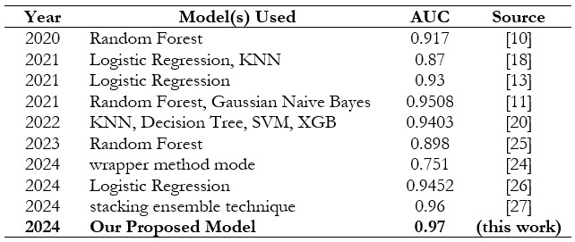
Using the UCI heart failure dataset, which contains 303 samples with fourteen attribute values, the researcher in [22] evaluated various machine learning algorithms, including Support Vector Machine, Random Forest, Naïve Bayes, Logistic scheme tree, K-Nearest Neighbor, and other information mining techniques. Among these algorithms, SVM has the highest score on accuracy of 84.1584 percent; others include decision tree, KNN, and Naive Bayes. Table 1 shows the results of the Area Under the Curve (AUC) for different machine learning models in the categorization of heart disease, ordered by AUC value. A well-balanced and optimized machine-learning approach for the detection of cardiac illness was suggested in [23].
Data description; training and testing datasets; attribute pruning; rule pruning; validation and prediction; suggested methodology; experimental setup; and lastly, the seven stages of the technique were carried out. The following information was considered: the Statlog heart database had 270 patients and 13 characteristics, while the Framingham dataset included 4240 patients and 15 attributes. On one hand, a cross-validation value of 10 and a random ratio of 9:1 was employed. Applying the BOML algorithm (in conjunction with Adasyn). The results showed an F1-Score of 80.7%, a recall of 83.2%, a precision of 79.00%, and a ROC curve of 78.00%. The authors use machine learning techniques to sift through many healthcare sources of data and generate sophisticated prediction models [24].
Table 1 summarizes the performance of various models used from 2020 to 2024 for predictive tasks, with AUC scores ranging from 0.812 to 0.97. Random Forest and Logistic Regression models frequently appear, demonstrating consistently high AUC scores, particularly in 2021 and 2023. The highest AUC scores were achieved by the stacking ensemble technique in 2024 with 0.96, and our proposed model in 2024, reached the top performance with an AUC of 0.97. This progression highlights the ongoing improvements in model performance over time.
Table 1. Summary of Previous Studies Compared to Our Study on Heart Disease Classification Methods
Dataset
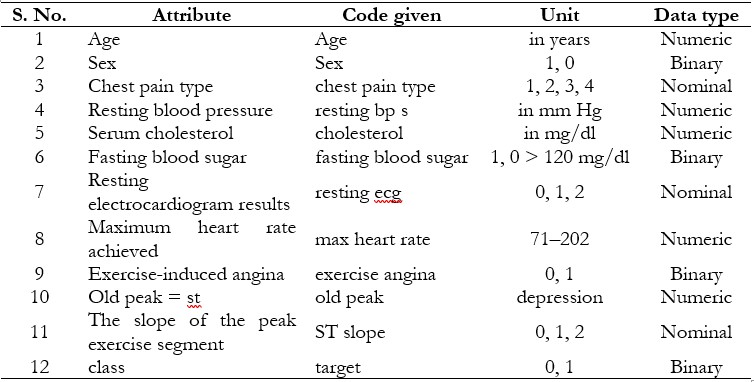
The heart disease classification dataset is an open-source resource available on Kaggle, making it valuable for machine learning research [8]. The Heart Disease dataset, originating from four locations Cleveland, Hungary, Switzerland, and Long Beach VA, comprises 76 attributes, including a target variable indicating the presence of heart disease (0 for no disease and 1 for disease). Table 2 shows a detailed discussion of our dataset [8]. Age, sex, type of chest pain, resting heart rate, levels of serum cholesterol, fasting blood sugar, heart rate maximum, exercise-induced chest pain, ST depression, thalassemia results, and a subset of eleven critical features are the most used features in many studies that utilize the complete dataset, which contains a vast array of patient information as presented in Table 3. Each feature provides critical information related to clinical and demographic factors that contribute to heart health. There are no data loss or completeness issues within any of the attributes which provides better analysis of values. Due to consideration of patient anonymity, the actual name and social security number have been removed and replaced as stand-ins.
Table 2. Dataset Details [8]
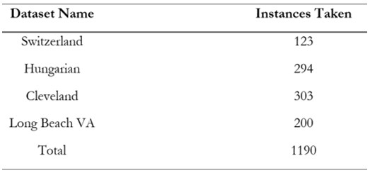
Machine learning algorithms are being created targeted to enhance the approaches to diagnosis and treatment of heart disease and, thus, the quality of patients’ lives. Additional details of these datasets and the number of instances are presented in Table 3.
Table 3. Heart Disease Dataset attribute description [28]
Methodology
In our research, we used a reduced dataset to set up ground control for a number of models. The first part of the work was aimed at revealing the basic behavior of every model and was helpful to compare with the results of further improved preprocessing. Since to begin with, we defined a set of basic features, after which none could attempt any challenging feature transformations or dimensionality reduction on the models, we make sure that the raw computing functionality and speed of the models could be properly assessed.
Due to the nature of our dataset, our method encompasses the analysis of several machine learning algorithms illustrated in Figure 6, by employing and excluding PCA. Each approach was assessed under two conditions: in the case of the original dataset and after transformation using PCA. For Logistic Regression, we looked at the implication of using dimensionality in terms of the predictive ability and the interpretability of the model. For the KNN algorithm both before and after PCA, to measure the impact of dimensionality reduction on the classification performance, the KNN algorithm was tested in its basic unmodified form. Overall, the effect of the dimensionality in applying the Naive Bayes model has been explored with and without PCA. Likewise, for investigating the effect of PCA on the Support Vector Machine (SVM) performance of classification, its execution was also examined. The Decision Tree model was initially applied with the raw dataset and the same model was also applied after applying PCA for affected features to identify the difference in outcomes due to feature reduction. Last but not least, we carried out the comparison between the Random Forest model that has undergone dimensionality reduction and the Random Forest model that has not, in other words, we looked at the impact of the dimensionality reduction technique on the Random Forest ensemble learning model.
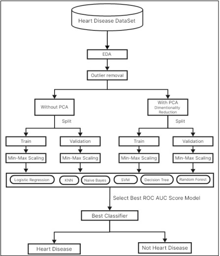
Figure 2. Workflow Diagram of Proposed Methodology
Data Preprocessing
Data Cleaning
In data preprocessing, the first step was to clean the Heart Disease Classification data so as to avoid the incorporation of poor-quality data. Our concentration was to pinpoint and solve any cases of missing values capable of affecting the ML algorithms’ performance. Ensuring that the dataset remained complete and reliable for analysis. After that, they cleaned the data and made a proper distinction between the independent variables and the dependent variables. It was important to take this step to determine which of those variables was used to predict heart disease risk.
Feature Encoding
In feature encoding, we transformed categorical variables into a numeric format that can be understood by machine learning algorithms. For example, the variables for the “chest pain type “and “sex” were encoded using one hot encoding where these categories were transformed to binary column format. This change made it possible for the algorithms to parse the data without any misinterpretation of the information.
Normalization
To improve the model’s performance, all the numerical features were scaled using Min-Max scaling after the input and output were split. This normalization technique made all the feature values fall within the same range mostly between 0 and 1. It was essential to do this scaling after the separation to avoid data leakage. If scaling were performed on the entire data before the split, then the model could learn something from the test set that is unwanted. This was accomplished by scaling only the training data and applying the same scaling parameters to that of the test set; hence, the assessment of the model was accurate and free from biases.
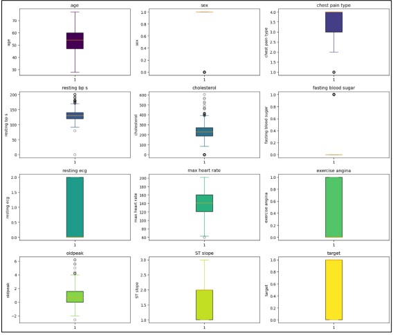
Figure 3. Outliers Detection.
Outlier Detection and Removal
We also cleaned the data to ensure that information that was not relevant or acted like an outlier, did not influence our results. Outliers are extreme values that might skew the results or break the assumptions of statistical measures and hence lead to erroneous conclusions and prognoses. To achieve a more precise identification of these outliers we used statistical tools such as the IQR, with the help of which it is possible to distinguish values that are outside the range of typical values. Also, to compare the result’s dispersion, we used boxplots, which are less formalized and make it easier to see outliers. For outlier identification which has been shown in the former discussion, the box plot shown in Figure 2 provides the most suitable means of visualizing the distribution of the numerical features while pointing out the outliers as well. This kind of visualization not only helps in viewing the spread of the data but also focuses on values that are beyond the normal range.
In Figure 3 the removal of outliers, we plotted a correlation heatmap of the numeric features within the dataset. This heatmap shown in Figure 4 is used to display linear relationships of different variables where the intensiveness of color illustrates the nature of the relationship. The individual points on the heatmap provide exact coefficients thus offering detailed inferential significance of how each feature influences others. We make this step important to diagnose multicollinearity and select features for predictive modeling to make the analysis more valuable.
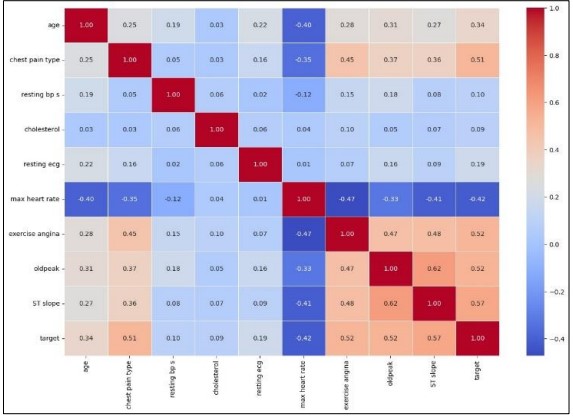
Figure 4. Correlation heatmap of numerical features after outlier removal.
Feature Extraction Using PCA
Principal Component Analysis (PCA) has the main role of dimensionality reduction of the given dataset while retaining as much of the valuable information as possible. PCA does this by mapping the original features into a new set of features that are orthogonal and known as principal components. These components have direction and amplitude in equal measure and as such can be used to represent the original data in a more compact manner because they contain maximum variance in the data. Since PCA concentrates on the main components, the impact of noise and redundancy is reduced, and the affectivity of subsequent modeling is improved. This transform is especially useful with large datasets such as the heart disease dataset, where the presence of many features may complicate the best fit. It is also important to note that using PCA not only helps in reducing dimensionality but also aids in enhancing the analysis and interpretation of the data.
In Figure 5 Dimensionality reduction was conducted using Principal Component Analysis (PCA) to achieve separation of most of the variance in lower dimensionality. The investigation considered up to 11 principle components and for each of them, the explained variance ratio was computed to assess the contribution of the component to the total variance. The plot of explained cumulated variance was used to display how variance builds up with each next component. The labels in this figure indicate the percentage of variance accounted for each component and ticks on the plot show the corresponding values. It shows that to model a large set of variables a small number of components is sufficient to capture a large part of the variance in the data which gives rather a clear indication of what number of components is needed to explain a given percentage of variance. For example, to achieve 99 percent variation, the research showed the number of components necessary indicating when effective dimensionality reduction should be implemented.
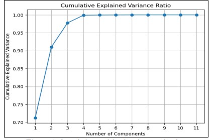
Figure 5. Cumulative explained variance ratio plot,
Figure 6 illustrates the relationship between the number of principal components and the total variance explained in the dataset. The marker indicates the optimal number of components needed to achieve a 99% variance explanation.
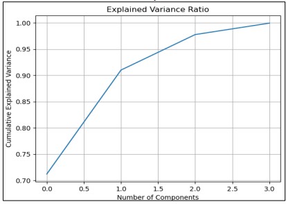
Figure 6. Cumulative Explained Variance Ratio for 3 Principal Components
In Figure 6 The variance is explained where the line graph shows the variance when PCA analysis is done with three components captures the variance within the dataset. The analysis of the dataset reveals that the first principal component accounts for the largest share of 90.88%, which indicates the ability of this component to represent most variation in the complete data set. The second primary measure, PC2, has 5.63% of the variance, and the third primary measure, PC3, explains 2.86%. A plot of the cumulative explained variance ratio against the number of components reveals that the first few components are highly significant in terms of the total variance. This visualization supports the fact that most of the variability is retained and most of the datasets can be represented with only a small number of principal components. Thus, the utilization of these three components gives a micro/Macro perspective of the data, which makes the analysis and interpretation straightforward.
Experimental Setup and Results
Experiment Setup
The experiments were performed on a high-performance computer, configuration with the following characteristics:
• CPU: AMD RYZEN 9 5900X
• GPU: NVIDIA GEFORCE RTX 4080 SUPER 16G
• VENTUS 3X OC
• Memory: 32 GB RAM
Logistic Regression Without PCA
We use the Logistic Regression model on the data originally without PCA in order to set benchmarks for its accuracy. Finally, Min-Max scaling was applied to the data, which was divided into trains and testing datasets then 10-fold Stratified Cross-Validation was performed to ensure validation. As for the average training accuracy and average test accuracy, the model can provide data of 82.67% and 80.78% respectively, so the model can be regarded as having a good result on both the training set and validation set. Importantly, the mean ROC AUC = 0.932, indicating a high measure in classification separation ability as presented in Figure 7. The training process which took a total of approximately 0.064 seconds was effectively completed. Confirming the model's practicality in terms of both accuracy and computational time.
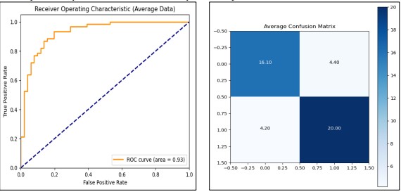
Figure 7. Performance Graphs with confusion Matrix for Logistic Regression (without PCA)
Logistic Regression with PCA
After using without PCA we used Logistic Regression with the PCA feature selection procedure, we reported the analyses of the different numbers of PCA components to be included in the model. The results were derived from a Min-Max scaled and standardized data set; PCA with the components 1 to 11 were included. For each configuration, we used 10-Stratification Cross-Validation to calculate accuracy, confusion matrix, and ROC AUC. The latter showed that using 10 PCA components was the most effective, with an average training accuracy of 83.23%, test accuracy of 82.13%, and ROC AUCs equal to 0.902. Using this configuration takes slightly above 0.05 seconds to begin the training process. This configuration gave a consistent and stable generalization of the accuracy and computational gain as observed from the different performance measures and the time utilization.
The final model which used 10 PCA components was re-trained, and the performance was tested using the test set confirming the high generalization performance of the model with a 0.91 ROC AUC score. The ROC curve and confusion matrix seen in Figure 8 presented that the applied model is accurate in classification.
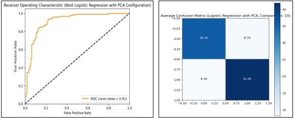
Figure 8. Performance Graphs with confusion Matrix for Logistic Regression (with PCA)
KNN Without PCA
In our analysis of K-Nearest Neighbors (KNN) with feature selection and hyperparameter tuning, we employed Grid Search Cross Validation using the range of the number of neighbors from 1 to 20. It was observed that the best setting for the output is achieved with the n_neighbors=11. In Figure 9 Averaged confusion matrix and ROC curves give the idea about the targeted model class effectiveness and performance indicators.
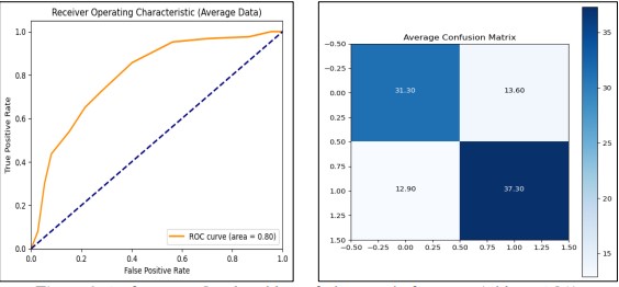
Figure 9. Performance Graphs with confusion Matrix for KNN (without PCA)
KNN with PCA
We evaluated the performance of the K-Nearest Neighbors (KNN) classifier combined with Principal Component Analysis (PCA) for dimensionality reduction. After splitting the dataset into training and test sets, and applying Min Max Scaler and Standard Scaler, we tested various PCA component counts ranging from 1 to 11. Our results indicated that using 11 PCA components achieved the highest average performance metrics, including a training accuracy of 89.1%, a test accuracy of 84.9%, and an ROC AUC score of 91.4%. The optimal configuration demonstrated robust classification capabilities and efficient training, taking only 0.38 seconds. These findings show that the combination of KNN with PCA effectively enhances model performance, with 11 components being the most advantageous for this dataset as presented in Figure 10.
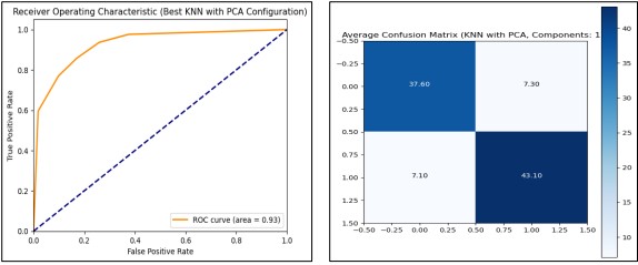
Figure 10. Performance Graphs with confusion Matrix for KNN (with PCA)
Naive Bayes Without PCA
Calculated Ten-fold cross-validations on the concerned data set using the Naive Bayes classifier of Gaussian kind in this exercise. Standard Scaler was applied to the dataset, and multiple significant measures were recorded, such as accuracy, confusion matrix, and ROC AUC score. The obtained values were approximately 83.8% for training data accuracy and 83.7% for test data accuracy. The average ROC AUC of the model was 90.4 while when the model was tested in the held-out test set, it got a slightly higher standard ROC AUC of 90.7. The training process, which took place as normalization, was finalized in about 0.05 sec. In Figure 11 confusion matrix and ROC curve give a comprehensive evaluation of the model’s performance.

Figure 11. Performance Graphs with confusion Matrix for Naive Bayes (without PCA)
Naive Bayes with PCA
Naive Bayes with Principal Component Analysis (PCA), as follows, discussed different numbers of PCA dimensionality for better predictions. The data set was normalized using the Min-Max Scaler function, after which Principal Component Analysis transformation was done and the data was normalized again. To evaluate performance in terms of different configurations of the PCA components, cross-validation on ten folds was used. The performance was presented for the case of using only 1 PCA component, after which the training accuracy was 76.9% on average, while the test accuracy was 76.98%. An average ROC AUC score of 87.97% derived from classes showed that classifiers performed well in terms of distinguishing classes. The training process of the PCA and normalization collectively required about 0.05 seconds.
In Figure 12 For each of the PCA component configurations, a confusion matrix was generated and plotted which offered quite specific information on the classification efficiency. With one PCA component, we reached the highest ROC AUC value, and further model refitting and evaluation restated the stability of this choice having a ROC AUC of 87.97%.

Figure 12. Performance Graphs with confusion Matrix for Naive Bayes (with PCA)
SVM Without PCA
The Support Vector Machine (SVM) model sets probability estimates to true to generate the ROC Curve and AUC. In this, we utilized Stratified K-Fold cross-validation with the number of folds set to 10 for each of the folds to preserve the ratio between the classes in the given dataset. The model across the folds obtains a training accuracy of.8690 and a test accuracy of.8423. Also, the model has an average ROC AUC score of 0.91 showing the ability of the model at different thresholds. We also derived the average confusion matrix for a better understanding of the model’s classification performance and understand where to improve as presented in Figure 13. Finally, the train model produced the ROC curve having the AUC 0.91.
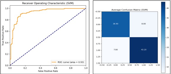
Figure 13. Performance Graphs for SVM with confusion Matrix (without PCA)
SVM with PCA
SVM model combined with PCA, we test the accuracy based on different numbers of PCA components. The first transformation methods include feature scaling using Min Max Scaler, as well as Standard Scaler to normalize the data in different ways. In the context of tuning parameters of the SVM model, Stratified K Fold cross-validation with 10 folds is used and reports indicate how the model performed for different numbers of PCA components. For each configuration, we store aspects like training accuracy data and test accuracy data, ROC AUC score, and confusion matrices. Most notably, the maximal result (11 PCA components) is the training accuracy of 91.48%, test accuracy of 87.60%, and ROC AUC of 0.93. The model trained and evaluated with this configuration is a model with the ability to classify as indicated by the ROC curve of the entire dataset. Figure 14 shows the evaluation process by adding PCA and improves the SVM model by optimizing the dimensionality with classification accuracy and AUC value.
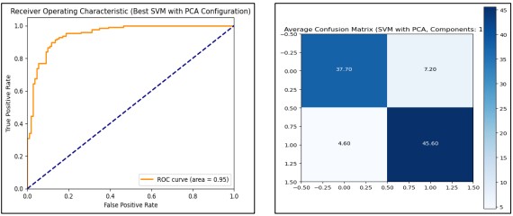
Figure 14. Performance Graphs with confusion Matrix for SVM (with PCA)
Decision Tree Without PCA
We subsequently employed a Decision Tree classifier; we went further to employ a 10-fold Stratified cross-validation for the purpose of testing. At each fold, the model was trained on one part of the data and validated on the other part, and the accuracy, confusion matrix, and ROC AUC score, were measured. The model reached 1.0 training accuracy and 0.873 testing accuracy suggesting the possibility of slight overfitting. Using an ROC AUC score of 0.91, In Figure 15, the model has a good classification ability between two classes. Next, after k-fold cross-validation, the model was retrained on the whole training set and tested on the test dataset for validation. This is another demonstration of how the model took only 0.057 seconds to train thereby exhibiting computational speed. To enhance generalization even more, it can be desirable to tweak other hyperparameters of the tree like max_depth or min_samples_split values, and compare with other models.
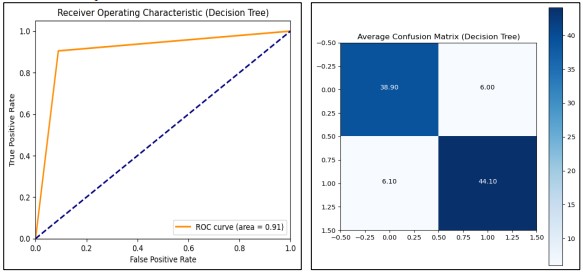
Figure 15. Performance Graphs with confusion Matrix for Decision Tree (without PCA)
Decision Tree with PCA
We analyzed the performance of a Decision Tree (DT) classifier when using a varying number of PCA components. To increase the accuracy and efficiency of the model the PCA was applied to the given dataset to remove the features that were not important. In each run, PCA components from 1 to 11 were used. The dataset was rescaled with Min Max Scaler then transformed using PCA and normalized. A K Fold cross-validation of Stratified type, with a set of 10 splits, was employed to ensure the model’s performance remained relatively stable regardless of the data splits. Mean training accuracy, mean test accuracy, and ROC AUC scores were used as the measures of evaluation. The expected 10-fold cross-validation model’s mean cross-validation accuracy was maximal when 8 PCA components were used, at 87.08% test accuracy and ROC AUC of 0.87 as presented in Figure 16. Thus, the final model was trained using the best of the above PCA parameters on the entire dataset and then validated once again on a new unseen test set to establish the effectiveness of the developed model in differentiating between patients with and without heart disease.
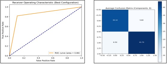
Figure 16. Performance Graphs with confusion Matrix for Decision Tree (with PCA)
Random Forest Without PCA
By using Random Forest, the model gave us a perfect average training accuracy of 1.0 meaning a perfect training on classification of the training data. Also, it demonstrated reasonable average test accuracy of approximately 91.38 % and a remarkable ROC AUC of 0.9626, to emphasize its high ability to classify data into classes. For the evaluation of model performance, we presented the AUC curve and confusion matrix in Figure 17.
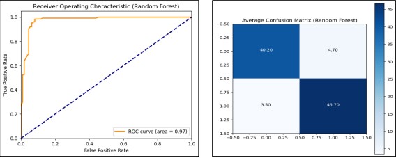
Figure 17. Performance Graphs with confusion Matrix for Random Forest (without PCA)
Random Forest with PCA
The evaluation of PCA component effectiveness shows that to attain the best performance, 11 components should be utilized for the Random Forest classifier with test accuracy around 90.33% and ROC AUC around 0.9616 shown in Figure 18.
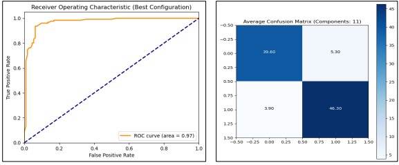
Figure 18. Performance Graphs with confusion Matrix for Random Forest (with PCA)
Following the steps of training and evaluating the Random Forest on the heart disease classification dataset, we proceeded to infer what the model will predict on similar new data. The model and scaler were directly loaded from the files and the dataset was preprocessed and scaled appropriately. Outcomes were predicted and odds were estimated for all instances. The results were saved, where besides the outcome of the given samples it contains the probability of heart disease. The confusion matrix was also calculated to visualize how well this model separates patients with and without heart disease. The analysis of these results is essential to determine the effectiveness of the model given the results attained in a practical real-world application. We evaluate the model on the new testing set of 256 instances and keep the old predictions for further analysis with other classification methods on the same dataset for the heart disease classification (Figure 19).
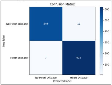
Figure 19. Visual representation of the Random Forest model’s classification performance
Discussion
In our study, traditional machine learning techniques were used mainly because of the nature of the data that we have used. The dataset is not so large, and we have well-defined features. Random Forest, Linear Logistic Regression, and Support Vector Machine are some of the typical models that are used, notably in a condition in which there is not much sample data to work with but there is a clear understanding of the domain features. By applying these techniques, we were able to train models without incurring a significant cost penalty relative to more highly complex methods that include deep learning, for equally reliable predictive accuracy. Consequently, we assessed the effects of activating PCA with diffident components with the classification of different machine-learning algorithms. These findings pointed out that the best number of components to be retained in the analysis was 11 according to the procedure of PCA. The result shows that when the Random Forest classifier is used on the dataset, it clearly improves its performance when it is preprocessed by the PCA algorithm. In all folds, the average train accuracy was 100% meaning that the model fits the training data well. Yet the test accuracy of 90.33% indicates that although the model is sound, optimization of generalization to the unseen data is achievable. Subjecting to the ROC AUC analysis, the derived score of 0.9616 holds strong evidence that the model is efficient in class discriminant, and lastly just under the model that has a score just below the perfect score of 0.97. This score indicates that the classifier has a high power for sorting out the positive from the negative instances which is desirable when working on problems where both sensitivity and specificity are important. From the selection of the PCA components, it was actually evident that the random forest model was whip-inspired.

Figure 20. Comparison Before Noise Removal
When the number of components was changed from 1 to 11, the PCA was able to capture more essential data variance thus increasing its predictive capability. Feature scaling was first conducted on all the features followed by application of the PCA technique and final normalization of the components. This strategy was effective in making the features ready for the Random Forest model since the algorithm requires good management of data complexity and data dimensionality. The new evaluation using the PCA with eleven components improved the ROC AUC score and test accuracy of the model when compared to previous evaluations using data that was not derived from PCA. This improvement reinforces the perception that dimensionality reduction can be useful in enhancing the performance of the models. The steps that were taken in the preprocessing phase including scaling, PCA transformation, and normalization proved to be a good framework that boosted the model. The time it took to train the model was approximately, 2.71 seconds when using the best configuration of the PCA. In this case, the time savings is a favorable result indicating that the model took a considerably short amount of time to train and evaluate while giving good results. The efficient time-used trains improve in real-world scenarios where model reactivity and elaborate capacity are valued. The comparison of all the models with ROC-AUC and training time is presented in Figure 20 and Figure 21.
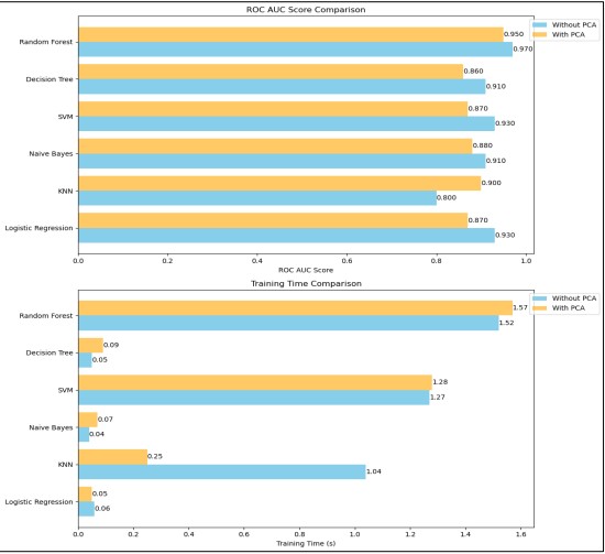
Figure 21. Comparison After Noise Removal
Conclusion
Conclusion and Future Work
Based on the performance of our proposed study, we have compared Random Forest, Logistic Regression, KNN, Naive Bayes, SVM, and Decision Tree in the context of the classification of heart diseases. After rigorous evaluation and benchmarking, the Random Forest algorithm showed the highest accuracy and ROC AUC score. PCA benefited the training by increasing the ROC AUC measure while simultaneously decreasing training time. Analyzing the results of our study we were able to show how dimensionality reduction and noise filtering affected model performance. In the future, for reliability, we will combine multiple diverse amounts of datasets to classify heart disease.
Acknowledgement
This study is being exclusively carried out by the authors while preparing the manuscript with their research interest and capacity and the research work was conducted at the Department of Computer Science, MNS University of Engineering and Technology, Multan, Pakistan. Department of Computer Science MNSUET contributed the research resource.
Author’s Contribution
All authors contributed equally to the conceptualization, design, implementation, and writing of this manuscript.
Conflict of Interest: The authors declare no conflict of interest regarding the publication of this manuscript in IJIST.
Reference
[1] “Cardiovascular diseases (CVDs).” Accessed: Oct. 21, 2024. [Online]. Available: https://www.who.int/news-room/fact-sheets/detail/cardiovascular-diseases-(cvds)?gad_source=1&gclid=CjwKCAjw1NK4BhAwEiwAVUHPUMwnj_ihnxxgw2el22_t5_Phxx8Gq4RcH5hl9J5rGxqnVjgLeDcUqhoCuKAQAvD_BwE
[2] R. Buettner and M. Schunter, “Efficient machine learning based detection of heart disease,” 2019 IEEE Int. Conf. E-Health Networking, Appl. Serv. Heal. 2019, Oct. 2019, doi: 10.1109/HEALTHCOM46333.2019.9009429.
[3] A. Singh and R. Kumar, “Heart Disease Prediction Using Machine Learning Algorithms,” Int. Conf. Electr. Electron. Eng. ICE3 2020, pp. 452–457, Feb. 2020, doi: 10.1109/ICE348803.2020.9122958.
[4] R. P. Choudhury and N. Akbar, “Beyond diabetes: a relationship between cardiovascular outcomes and glycaemic index,” Cardiovasc. Res., vol. 117, no. 8, pp. e97–e98, Jul. 2021, doi: 10.1093/CVR/CVAB162.
[5] “Ischemic Heart Disease Statistics 2024 By Risk, Factor, Treatments.” Accessed: Oct. 21, 2024. [Online]. Available: https://media.market.us/ischemic-heart-disease-statistics/
[6] K. Shameer, K. W. Johnson, B. S. Glicksberg, J. T. Dudley, and P. P. Sengupta, “Machine learning in cardiovascular medicine: are we there yet?,” Heart, vol. 104, no. 14, pp. 1156–1164, Jan. 2018, doi: 10.1136/HEARTJNL-2017-311198.
[7] J. P. Li, A. U. Haq, S. U. Din, J. Khan, A. Khan, and A. Saboor, “Heart Disease Identification Method Using Machine Learning Classification in E-Healthcare,” IEEE Access, vol. 8, pp. 107562–107582, 2020, doi: 10.1109/ACCESS.2020.3001149.
[8] “Human Heart Disease dataset.” Accessed: Oct. 21, 2024. [Online]. Available: https://www.kaggle.com/datasets/tejpal123/human-heart-disease-dataset/data
[9] A. U. Haq, J. Li, M. H. Memon, M. Hunain Memon, J. Khan, and S. M. Marium, “Heart Disease Prediction System Using Model of Machine Learning and Sequential Backward Selection Algorithm for Features Selection,” 2019 IEEE 5th Int. Conf. Converg. Technol. I2CT 2019, Mar. 2019, doi: 10.1109/I2CT45611.2019.9033683.
[10] Y. Lin, “Prediction and Analysis of Heart Disease Using Machine Learning,” 2021 IEEE Int. Conf. Robot. Autom. Artif. Intell. RAAI 2021, pp. 53–58, 2021, doi: 10.1109/RAAI52226.2021.9507928.
[11] P. Motarwar, A. Duraphe, G. Suganya, and M. Premalatha, “Cognitive Approach for Heart Disease Prediction using Machine Learning,” Int. Conf. Emerg. Trends Inf. Technol. Eng. ic-ETITE 2020, Feb. 2020, doi: 10.1109/IC-ETITE47903.2020.242.
[12] H. El Hamdaoui, S. Boujraf, N. E. H. Chaoui, and M. Maaroufi, “A Clinical support system for Prediction of Heart Disease using Machine Learning Techniques,” 2020 Int. Conf. Adv. Technol. Signal Image Process. ATSIP 2020, Sep. 2020, doi: 10.1109/ATSIP49331.2020.9231760.
[13] H. Kumar Thakkar, H. Shukla, and S. Patil, “A Comparative Analysis of Machine Learning Classifiers for Robust Heart Disease Prediction,” 2020 IEEE 17th India Counc. Int. Conf. INDICON 2020, Dec. 2020, doi: 10.1109/INDICON49873.2020.9342444.
[14] D. Rahmat, A. A. Putra, Hamrin, and A. W. Setiawan, “Heart Disease Prediction Using K-Nearest Neighbor,” Proc. Int. Conf. Electr. Eng. Informatics, 2021, doi: 10.1109/ICEEI52609.2021.9611110.
[15] N. Basha, S. P. Ashok Kumar, C. Gopal Krishna, and P. Venkatesh, “Early Detection of Heart Syndrome Using Machine Learning Technique,” 4th Int. Conf. Electr. Electron. Commun. Comput. Technol. Optim. Tech. ICEECCOT 2019, pp. 387–391, Dec. 2019, doi: 10.1109/ICEECCOT46775.2019.9114651.
[16] W. M. Jinjri, P. Keikhosrokiani, and N. L. Abdullah, “Machine Learning Algorithms for the Classification of Cardiovascular Disease- A Comparative Study,” 2021 Int. Conf. Inf. Technol. ICIT 2021 - Proc., pp. 132–138, Jul. 2021, doi: 10.1109/ICIT52682.2021.9491677.
[17] P. Sujatha and K. Mahalakshmi, “Performance Evaluation of Supervised Machine Learning Algorithms in Prediction of Heart Disease,” 2020 IEEE Int. Conf. Innov. Technol. INOCON 2020, Nov. 2020, doi: 10.1109/INOCON50539.2020.9298354.
[18] S. Hameetha Begum and S. N. Nisha Rani, “Model Evaluation of Various Supervised Machine Learning Algorithm for Heart Disease Prediction,” Proc. - 2021 Int. Conf. Softw. Eng. Comput. Syst. 4th Int. Conf. Comput. Sci. Inf. Manag. ICSECS-ICOCSIM 2021, pp. 119–123, Aug. 2021, doi: 10.1109/ICSECS52883.2021.00029.
[19] B. P. Doppala, D. Bhattacharyya, M. Janarthanan, and N. Baik, “A Reliable Machine Intelligence Model for Accurate Identification of Cardiovascular Diseases Using Ensemble Techniques,” J. Healthc. Eng., vol. 2022, no. 1, p. 2585235, Jan. 2022, doi: 10.1155/2022/2585235.
[20] R. Tao et al., “Magnetocardiography-Based Ischemic Heart Disease Detection and Localization Using Machine Learning Methods,” IEEE Trans. Biomed. Eng., vol. 66, no. 6, pp. 1658–1667, Jun. 2019, doi: 10.1109/TBME.2018.2877649.
[21] N. Louridi, M. Amar, and B. El Ouahidi, “Identification of Cardiovascular Diseases Using Machine Learning,” 7th Mediterr. Congr. Telecommun. 2019, C. 2019, Oct. 2019, doi: 10.1109/CMT.2019.8931411.
[22] “Prediction of Heart Diseases Using Data Mining and Machine Learning Algorithms and Tools.” Accessed: Oct. 21, 2024. [Online]. Available: https://www.researchgate.net/publication/324162326_Prediction_of_Heart_Diseases_Using_Data_Mining_and_Machine_Learning_Algorithms_and_Tools
[23] A. J. Albert, R. Murugan, and T. Sripriya, “Diagnosis of heart disease using oversampling methods and decision tree classifier in cardiology,” Res. Biomed. Eng., vol. 39, no. 1, pp. 99–113, Mar. 2023, doi: 10.1007/S42600-022-00253-9/FIGURES/13.
[24] A. H. Elmi, A. Abdullahi, and M. A. Barre, “A machine learning approach to cardiovascular disease prediction with advanced feature selection,” Indones. J. Electr. Eng. Comput. Sci., vol. 33, no. 2, pp. 1030–1041, Feb. 2024, doi: 10.11591/ijeecs.v33.i2.pp1030-1041.
[25] T. R. Ramesh, U. K. Lilhore, M. Poongodi, S. Simaiya, A. Kaur, and M. Hamdi, “PREDICTIVE ANALYSIS OF HEART DISEASES WITH MACHINE LEARNING APPROACHES,” Malaysian J. Comput. Sci., vol. 2022, no. Special Issue 1, pp. 132–148, Mar. 2022, doi: 10.22452/MJCS.SP2022NO1.10.
[26] M. Nasiruddin, S. Dutta, R. Sikder, M. R. Islam, A. AL Mukaddim, and M. A. Hider, “Predicting Heart Failure Survival with Machine Learning: Assessing My Risk,” J. Comput. Sci. Technol. Stud., vol. 6, no. 3, pp. 42–55, Aug. 2024, doi: 10.32996/JCSTS.2024.6.3.5.
[27] S. Mondal, R. Maity, Y. Omo, S. Ghosh, and A. Nag, “An Efficient Computational Risk Prediction Model of Heart Diseases Based on Dual-Stage Stacked Machine Learning Approaches,” IEEE Access, vol. 12, pp. 7255–7270, 2024, doi: 10.1109/ACCESS.2024.3350996.
[28] N. A. J. -, Z. J. P. -, and R. M. -, “Cardiovascular Disease (CVD) Prediction Using Machine Learning Techniques With XGBoost Feature Importance Analysis,” IJFMR - Int. J. Multidiscip. Res., vol. 5, no. 5, Oct. 2023, doi: 10.36948/IJFMR.2023.V05I05.7715.
