Addressing Illicit Tobacco Growth in Pakistan: Leveraging AI and Satellite Technology 
for Precise Monitoring and Effective Solutions

Waleed Khan; Nasru Minallah; Atif Sardar Khan

Addressing Illicit Tobacco Growth in Pakistan: Leveraging AI and Satellite Technology for Precise Monitoring and Effective Solutions

Khan. W^1*,2,Minallah. N^1,2,Khan. A. S³

¹Department of Computer Science & Information Technology, University of Engineering and Technology, Peshawar, Pakistan

²National Center for Big Data and Cloud Computing (NCBC), University of Engineering and Technology, Peshawar, Pakistan.

³Department of Renewable Energy Engineering, University of Engineering and Technology Peshawar, Pakistan

Abstract
The market share of illicit tobacco products in Pakistan has seen a significant surge in recent years. In 2022, it reached a staggering 42.5%. Since January 2023, there has been a sharp 32.5% increase in volumes of Duty Not Paid (DNP) products and a remarkable 67% surge in the quantities of smuggled cigarettes. This rise can be attributed to the unregistered and unlicensed tobacco cultivation in Pakistan. This sector has largely relied on conventional methods for data collection in the field, primarily managed by the country's crop statistical departments. The utilization of cutting-edge artificial intelligence techniques and satellite imagery for generating crop statistics has the potential to address this issue effectively. We established a synergy by combining images from two remote sensing satellites and collected field data to detect tobacco crops using Recurrent Neural Networks (RNN). The results affirm the effectiveness of these techniques in detecting and estimating the acreage of tobacco crops in the observed areas, particularly in a union council of the Swabi region. We conducted surveys to collect training and validation data through our proprietary smartphone application, GeoSurvey. The collected data was subsequently refined, preprocessed, and organized to prepare it for use with our deep learning algorithm. The model we developed for the detection and acreage estimation of tobacco crops is called Convolutional Long Short-Term Memory (ConvLSTM). We created two datasets from the acquired satellite images for comparison. Our experimentation results demonstrated that the use of ConvLSTM for the synergy of Sentinel-2 and Planet-Scope imagery yields higher training and validation accuracy, reaching 98.09% and 96.22%, respectively. In comparison, the use of time series Sentinel-2 images alone achieved training and testing accuracy of 97.78% and 95.56%

Keywords: Tobacco, Artificial Intelligence, Deep Learning, Recurrent Neural Networks, Remote Sensing, Sentinel-2,Planet-Scope

Corresponding Author	How to Cite this Article
Waleed Khan,Department of Computer Science & Information Technology, University of Engineering and Technology, Peshawar, Pakistan	Waleed Khan, Nasru Minallah, Atif Sardar Khan, Addressing Illicit Tobacco Growth in Pakistan: Leveraging AI and Satellite Technology for Precise Monitoring and Effective Solutions. IJIST. 2023 ;5(4):424-439 https://journal.50sea.com/index.php/IJIST/article/view/549

Introduction

Tobacco cultivation holds significant economic importance in Khyber Pakhtunkhwa (KP), Pakistan, involving a substantial workforce and yielding an annual production of 100,000 tons. The profits generated from tobacco farming are considerable, and it is in high demand among cigarette manufacturers. Agriculture, including tobacco cultivation, contributes around 21% to the country's Gross Domestic Product (GDP) [1], with KP accounting for a substantial 55% of the national tobacco production. In Pakistan, traditional techniques are used for monitoring tobacco plantations. These techniques are human-centric and require many surveyors to monitor and take records. Most of the tobacco fields are left out in these surveys. However, accurately estimating tobacco crops has become a challenge for government data analysts. This inaccuracy has resulted in significant losses in tax revenue and the proliferation of illicit tobacco production, which has notably surged over the past five years [2]. The primary cause of this unlawful growth of tobacco can be linked to tax evasion. Farmers must acquire a license from government bodies to regulate the cultivation of excess tobacco on plantations, they unlawfully plant tobacco crops just to bypass this phase. The data illustrating the market share of illicit tobacco from 2010 to 2022, as shown in Figure 1, exhibits a noticeable pattern of fluctuations. In 2010, illicit tobacco accounted for 18.90% of the market share, and this percentage witnessed a gradual increase in the following years. There was a substantial spike, with illegal tobacco comprising 40.60% of the market by 2016, followed by a slight increase up to 41.20% by 2017. There has been a decline in the market share of unauthorized tobacco at the start of the year 2018, with some fluctuations but it showcased an overall downward trend. However, in 2022, this share increased up to 42.50%. Understanding these variations is crucial for policymakers and authorities to implement effective measures to combat the furtive tobacco trade. A recent report published by the Pakistan Bureau of Statistics (PBS) stated a loss of Rs. 240 billion annually due to unlicensed tobacco products in the market.

There has been a considerable amount of work done to ensure the sale of illegal tobaccobased products, top in the line are cigarettes. Developed countries with mainstream systems have started the use of advanced technologies like high-tech packaging, labeling, and track and trace systems, but still, at the time of plantation, there needs to be a system powered by AI and satellite technology.

To address this issue, Remote Sensing (RS) technology, which employs satellites to observe Earth from space, can be a valuable tool [3]. There is a pressing need to develop advanced Artificial Intelligence (AI) algorithms for generating accurate crop statistics, particularly for crops like tobacco. One effective approach involves Neural Networks-based models for crop classification. To tackle the issues related to obtaining precise crop statistics for governmental statistical bodies, it is crucial to explore innovative research methods aimed at resolving these issues. The incorporation of RS technology along with advanced neural network algorithms, including Convolutional Neural Networks (CNN) and RNN. There are several advantages as well as challenges in implementation of such a system. These include;

Advantages of AI and Satellite Technology:

 Enhanced surveillance and quick detection

 Cost-effective solution

 Combat tax evasion and environmental impact

 Precision in detection and support for law enforcement

Challenges in Implementing Technology:

 Privacy concerns and accuracy issues

 Initial setup costs and technical expertise

 Adapting illicit growers

 Legal and ethical considerations

Figure 1: Illicit tobacco market share over the past decade

Related Work:

Utilizing the synergy between the Global Navigation Satellite System (GNSS) and Geographic Information System (GIS) enables an improved assessment of the variations in agricultural fields. This integration combines accurate positioning data from GNSS with the spatial analysis capabilities of GIS, leading to a deeper understanding of the diversity within these fields [4]. RS satellites offer a diverse array of features, including multiple channel options with specific wavelengths, varying spatial, temporal, and spectral resolutions, as well as different revisit times. Currently, RS satellites play a pivotal role in the detection, monitoring, and estimation of various aspects of crops, encompassing their health, growth status, and maturity [5] [6]. Numerous satellites, such as GeoEye-1, Ikonos, Formosat-2, Advanced Land Observation System (ALOS), SPOT 6, and SPOT 7, have been purposefully developed for the task of agricultural monitoring. These satellites enable precise analysis of crop health, vegetation detection, and drought mapping [7][8]. The deployment of ESA's Sentinel-2A and Sentinel-2B sibling RS satellites in 2015 and 2017, respectively, marked a notable advancement in the accessibility of open data for RS applications. These Sentinel-2 satellites furnish Multispectral Images (MSI) that encompass a total of 13 spectral bands. The temporal frequency of Sentinel- 2 satellites is noteworthy, as they return to similar locations on Earth every 5 days. This rapid revisit rate ensures consistent and frequent monitoring of dynamic processes, including changes in vegetation growth and alterations to the land surface. The increased temporal resolution greatly enhances our ability to monitor and analyze time-sensitive phenomena in various environmental and agricultural contexts [9].

Planet-Scope is a well-recognized commercial fleet of multispectral satellites renowned for its high-resolution imagery. Under Planet's management, this satellite constellation plays a pivotal role as a valuable source of Earth observation data. Planet-Scope Satellites (PSS) capture multispectral images with impressive detail, allowing for in-depth analysis and continuous monitoring of the Earth's surface [10].

RS has found extensive application among researchers for conducting both quantitative and qualitative assessments of tobacco crops. This approach is particularly favored for its userfriendly interface, rapid task completion, cost-effectiveness, and eco-friendliness. Nonetheless, it is crucial to consider variables such as the quality of RS data, the specific sensor utilized, and the chosen analysis methodologies, as these factors can influence the accuracy and reliability of the obtained results.

Liao et al. employed a DL model to delineate agricultural zones in Southwestern Ontario. They utilized multi-temporal polarimetric Synthetic Aperture Radar (SAR) and available multispectral RS data for crop classification. This study introduced the use of a one-dimensional Convolutional Neural Network (CNN) and suggested that the optimal crop classification results were achieved by combining multispectral data from VENµS and RADARSAT-2 through the Minimum Noise Fraction (MNF) transformation [11].

Zhang et al. compiled spectral data encompassing 16 different crop species across various experimental scenarios [12]. Systematically, they built a spectral database to aid the assessment of crop classification techniques and continuous monitoring of crop status. Their approach involved the utilization of observations based on JM distance and ISODATA for Random Forest (RF) [13], K-Nearest Neighbor (KNN), and Support Vector Machine (SVM) [14]. Their methodology played a pivotal role in the establishment of a comprehensive plant spectral library.

For tobacco crop detection, several multi-step algorithms have been proposed. In [15], Sun et al. introduced a two-step CNN approach that utilized RGB images to classify them into tobacco and non-tobacco fields.

Palchowdhuri et al. presented a three-step algorithm [16]. Their method involved the integration of high and very-high-resolution images, the computation of various Vegetation Indices (VIs), and ultimately, classification using a combination of algorithms. They incorporated multispectral and hyperspectral images with limited temporal data, sourced from three images of Coalville (UK) captured by Sentinel-2 and WorldView-3 [17] during the period from April to July 2016. Three VIs, specifically the Normalized Difference Vegetation Index (NDVI) [18], Soil-Adjusted Vegetation Index (SAVI) [19], and green NDVI (GNDVI) were derived from the red, green, and Near-Infrared (NIR) bands. Following this, they conducted supervised image classification using a combination of Decision Tree (DT) [20]and Random Forest (RF) algorithms.

In their study, Fan et al. employed images captured by Unmanned Aerial Vehicles (UAVs) in fourteen tobacco-growing regions to identify and count tobacco plants [21]. The researchers developed a three-step algorithm based on DNN. These steps involved plant extraction, subsequent classification into tobacco and non-tobacco plants, and post-processing of the classified images.

In their efforts to classify plantation regions, they implemented watershed segmentation as a method to delineate areas with tobacco plants from those devoid of them, contributing to a more precise categorization. Afterward, a CNN was trained using the segmented data to perform the classification task. Finally, post-processing was conducted to remove non-tobacco regions. This approach achieved an impressive overall accuracy rate of 91%. In recent years, there has been a significant increase in the popularity of DL models, particularly Artificial Neural Networks (ANNs) that are distinguished by their multiple hidden layers. This growing interest is driven by ANNs' remarkable ability to understand and learn endto-end data representations, reducing the need for manual feature extraction based on human expertise and experience [22][23].

DL has risen to prominence as a revolutionary technology in the fields of Machine Learning (ML), data mining, and RS science [24]. This ascent is primarily attributed to the versatility of DL models, their ability to autonomously learn without the need for expert supervision, computational efficiency, and their exceptional capability to represent features, particularly in the context of image classification [25]. [8] highlighted the remarkable utility of Sentinel-2 and Planet-Scope Dove imagery, renowned for their exceptionally high spatial resolution. These images were effectively employed to extract information about various vegetation phenology stages, even in challenging terrains characterized by short-term vegetation seasons. To discern between different phases of crop growth, they introduced an innovative approach that incorporates spatiotemporal RS images and employs 3D CNNs instead of conventional 2D CNNs for crop classification [26].

Among the various types of Recurrent Neural Network (RNN) models, Long ShortTerm Memory (LSTM) has established itself as highly effective in managing sequential data challenges [27][28]. LSTMs are purposefully designed to address the intricacies of long-term dependencies between events with temporal gaps, excelling in the acquisition and retention of information [29]. Notably, unlike Simple Recurrent Neural Networks (SRNNs), LSTMs do not grapple with significant optimization hurdles [30]. Consequently, LSTM models are exceptionally well-suited for a wide array of applications, including tasks such as speech synthesis, handwriting recognition, language translation, and the analysis of audio and video data [31][32][33].

Figure 2: Operational procedure of the utilized technique operational

A substantial amount of information is required to gather the necessary data for training DL models. Surveys were conducted in tobacco-growing regions to collect Ground Truth Data (GTD) to address this requirement. Additionally, satellite data from sources like Sentinel-2 and Planet-Scope were used for in-depth analysis. Once the model was trained, it underwent validation tests using test data and validation surveys to ensure its accuracy. This integrated approach has the potential to tackle the issue of illegitimate tobacco growth, enhance the accuracy of crop statistics, and provide benefits to both the government and the economy. Figure 2 illustrates the procedural diagram of the steps employed in this research. Ground truth surveys were conducted in four districts to collect tobacco and other vegetation data in the form of shapefiles, which were then refined through our in-house data preprocessing platform, Geo Survey Web. Satellite data from Sentinel-2 was obtained from the ESA Copernicus data hub. These images underwent preprocessing for geometric and radiometric correction. The refined data from the surveys was overlaid onto the preprocessed Sentinel-2 image time series data to record training pixels for different classes in the Sentinel-2 time series images. This data was subsequently fed into CNN and LSTM networks for crop categorization. The study employed various accuracy metrics, including Precision, Recall, Overall Accuracy, and F1-Score.

Study Site:

GTD was obtained from four distinct locations to ensure data diversity. These regions encompass Chotalahor, Charbagh, Mandani, and Yarhussain. However, the pilot region selected for testing purposes is Dobian, a tehsil in the Swabi district (Figure 3).

Figure 3: Study site under observation

Objectives:

 The primary objective of this study is to propose effective measures for curbing illicit tobacco crop growth in Pakistan.

 To outline the methodology for estimating tobacco crops utilizing satellite imagery.

 To formulate a state-of-the-art deep learning algorithm for accurate land use and land cover classification.

Novelty:

This research introduces the implementation of cutting-edge RNN to address the urgent problem of unlawful tobacco growth in Pakistan. It leverages satellite data, combining information from two distinct satellite systems: Sentinel-2 and Planet-Scope. The ConvLSTM model is employed to train and evaluate the model using field-collected data, representing a novel approach to satellite-based crop statistics generation.

Material and Method

The study encompasses the execution of experiments utilizing two sets of field-collected data. Table 1 delineates these two configurations for the experimental setups. Data from five dates of Sentinel-2 were harnessed to construct a concise temporal frame for May 2022. Sentinel- 2 provided 10 bands with spatial resolutions of 10 and 20 meters. The experimental configuration was devised with consideration for these data channels from both satellites. Setup-S2only has complete bands of Sentinel-2 and Planet-Scope, with varying resolutions, i.e., from 10 meters to 20 meters, while Setup-PS-S2cat contains data channels from Senitnel-2 and Planet-Scope. This is to test and compare the performance of data channels based on their resolutions.

Table 1: Datasets generated for the experiments.

Ground Truth Data:

The GTD collected during ground truth surveys in three districts, Swabi, Charsadda, and Mardan, was divided between training and testing datasets. The models were trained on the training data, while the testing data, which the model had never seen before, was used for validation purposes. The data was split with a proportion of 70% for training and 30% for testing, as shown in Table 2.

Table 2: Proportion of Training and Testing Data Split

Deep Learning Architectures:

The operational procedures of employed architectures and the fine-tuning of hyperparameters are elaborated here. The results have been obtained through thorough hyperparameter tuning, primarily carried out through an iterative trial-and-error process, which aligns with the nature of Neural Networks (NN). The experiments were conducted using the following architectural configurations.

Long Short-Term Memory (LSTM):

LSTM, represents a specialized type of RNN designed to excel in processing sequential data while retaining critical information over extended timeframes. It stands as an advanced evolution of RNNs, primarily distinguished by its ingenious solution to the vanishing gradient problem often encountered in traditional RNN training. The key innovation within LSTMs is their utilization of a gating mechanism, which selectively updates and retains information, granting them the capability to effectively capture and utilize data over prolonged periods. The credit for the development of LSTM networks goes to Sepp Hochreiter and Jürgen Schmidhuber, who introduced this concept in a seminal paper published in 1997 [27]. Subsequently, numerous researchers, including notable figures like Alex Graves, Felix Gers, and Jurgen Schmidhuber himself, have made substantial contributions to refining and popularizing LSTM networks. These networks have demonstrated exceptional effectiveness across a wide array of applications and have achieved extensive adoption in diverse fields.

LSTM networks offer a compelling solution to address the persistent challenge known as the vanishing gradient problem, a common issue encountered in traditional RNNs. They achieve this by incorporating feedback connections that enable them to retain crucial information over prolonged periods. LSTMs exhibit a versatile nature, capable of processing both individual data points, such as images, and entire sequences of data, including applications in speech or video analysis. These networks have found practical utility in a range of tasks, spanning unsegmented, connected handwriting recognition, speech recognition, and the detection of anomalies in network traffic or Intrusion Detection Systems (IDSs).

A significant advantage of LSTMs lies in their ability to adeptly capture long-term temporal dependencies, surpassing many other neural network architectures in this regard, all while circumventing the intricacies of optimization. This unique capability has elevated LSTMs to a prominent position in tasks where preserving the sequential order of information is of utmost importance. Notable applications include natural language processing, video analysis, and the forecasting of time-series data. A schematic diagram of LSTM is presented in Figure 4. In contrast to a typical RNN, LSTM incorporates an extended memory module explicitly designed to maintain critical information for subsequent layers. Each LSTM layer includes a Long Memory unit, often referred to as the Cell State. The core concept behind LSTMs is centered on the utilization of gates. These gates act as crucial control mechanisms, determining whether to preserve or update new features based on the model's requirements.

Figure 4: Schematic diagram of LSTM

Convolutional LSTM:

In the realm of image processing, a commonly employed technique to enhance or refine images and achieve specific desired results involves the application of filters [34]. These filters function as tools for emphasizing features or extracting valuable information from images (Figure 5). The process begins with the creation of a filter, such as a high-pass filter, which is then systematically applied to the image. The result is an image that retains only the relevant information while filtering out low-frequency pixels. Typically, these filters are configured as windows with dimensions NxM, where N represents the number of rows, and M represents the number of columns.

In the context of NN these filters are employed for feature extraction from images [35]. These extracted features often encompass attributes like edges, textures, and patterns, serving as distinctive markers for objects within the image under consideration.

Figure 5: Image convolution using a 3x3 kernel (Courtesy of Bi-Min Hsu)

Convolutional LSTM is an ANN architecture that blends convolutional and LSTM layers to model spatial and temporal dependencies in data. It is a modified version of the conventional LSTM network and is employed for processing sequential data such as time series or videos. The convolutional layer within the network is used to process the spatial details of the input data, whereas the LSTM layer is responsible for capturing temporal dependencies over time (Figure 6). The integration of these layers enables the Convolutional LSTM to process intricate sequences of spatial and temporal data with improved precision and efficacy, making it an extremely useful tool in various applications such as speech recognition, autonomous driving, and video analysis. The employed model for ConvLSTM is provided below in Figure 6.

Figure 6: Designated model of ConvLSTM

Result and Discussion

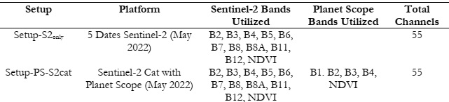
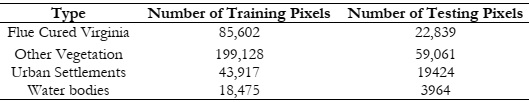
This section represents the impactful results obtained from our experiments conducted on the datasets central to our study, listed in Table 1 Datasets are used with ConvLSTM and their results are compared systematically. The collected GTD is split into training and testing data with a ratio of 70% and 30% for training and testing data respectively (Table 2). The testing data is completely unseen for the model and thus represents separate crop fields instead of pixels. This measure is taken to ensure generalization in the model.

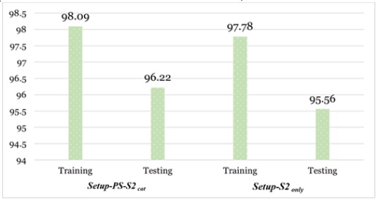
As illustrated in Figure 7 below, Setup-PS-S2cat outperforms Setup-S2only, attaining an overall training and testing accuracy of 98.09% and 96.22% respectively. Looking at the training and testing accuracy of Setup-S2only, it can be observed that 96.18% and 93.43% accuracies are achieved respectively.

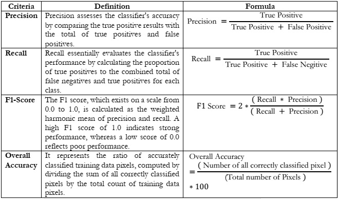
Accuracy Metrics Employed for Assessment:

Classification evaluation criteria employed are listed in Table 3.

Table 3: Evaluation criteria for classification of results

Figure 7: Overall accuracies of ConvLSTM for Setup-PS-S2cat and Setup-S2onl

Figure 8: Model accuracy and model loss for Setup-S2only

Table 4: Classification report of testing data for Setup-S2only

Setup-PS-S2cat:

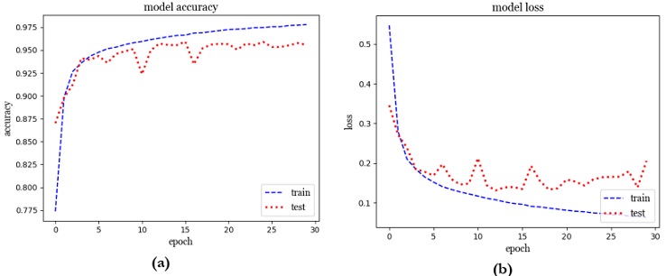
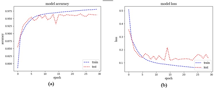
Throughout the 30 epochs of training depicted in Figure 9(a) and Figure 9(b), the model demonstrated consistent improvement. It began with an initial loss of 0.5106 and an accuracy of 78.50%, steadily progressing to an impressive accuracy of 98.09% by the end of the training process. Concurrently, the loss steadily decreased from 0.5106 to 0.0541, highlighting the model's improved performance. This progress extended to the validation set as well, where accuracy increased from 85.49% to 96.22%. In tandem, the validation loss dropped significantly from 0.3539 to 0.1325, indicating enhanced generalization. 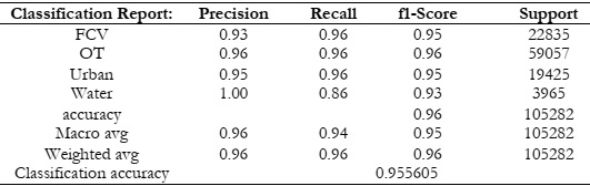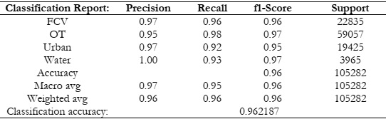The model's training journey showcased consistent enhancements in accuracy and reduced loss, affirming its effective learning and robust performance. The classification report in Table assesses four classes: FCV, OT, Urban, and Water. Notably, precision values are high, ranging from 0.95 to a perfect 1.00, indicating accurate positive predictions. The model's recall values, ranging from 0.92 to 0.98, show its ability to correctly identify actual instances. Balanced precision and recall result in impressive F1-scores between 0.95 and 0.97, affirming overall effectiveness in classification. The model's accuracy is strong at 0.96, indicating 96% correct classifications. The classification accuracy value of 0.962187 underscores its reliability in predicting class labels.

Figure 9: Model Accuracy and Model Loss for Setup-PS-S2cat

Table 5: Classification report of testing data for Setup-PS-S2cat

Setup-PS-S2cat vs Setup-S2only:

In the comparison between Setup-S2only and Setup-PS-S2cat, especially concerning the FCV class, it becomes evident that Setup-PS-S2cat boasts several advantages. First, Setup-PSS2cat exhibits a higher precision (0.97) compared to Setup-S2only (0.93), indicating its superior ability to make accurate positive predictions for the FCV class. Additionally, both models share the same recall (0.96), which means they correctly identified an equal proportion of actual FCV instances. However, the strong point for Setup-PS-S2cat becomes more apparent when considering the F1-score, where it achieves 0.96, indicating a better balance between precision and recall. In contrast, Setup-S2 only has an F1-score of 0.95 for the FCV class. Setup-PS-S2cat demonstrates stronger performance in accurately identifying and classifying instances of the FCV class, as it achieves higher precision and a slightly better F1-score compared to Setup-S2only. 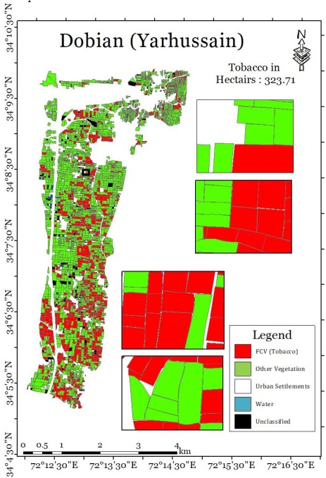The classification map of Dobain (Yarhussain) is provided in Figure 11.

Significance of the results achieved through Setup-PS-S2cat:

The effective utilization of multi-satellite data in our experimental setup lay out a plan for accurate estimation of tobacco crop acreage in a vast geographical area. In addition, the usage of temporal data from Sentinel-2 and Planet-Scope enhances the classification results with efficiency. To ensure further validation of our classification results (depicted in Figure 11) validation surveys have been carried out in the pilot region for pinpointing False positives and True Negatives. The classification map provided in Figure 11 presents ConvLSTM results with 4 classes; Tobacco (Red), Other Vegetation (Green), Urban (White), and Water (Blue). It can be seen from the figure that Tobacco plantations are clearly distinguishable from other classes. Our findings from the validation surveys validate DL model results with the same accuracy as presented in Table .

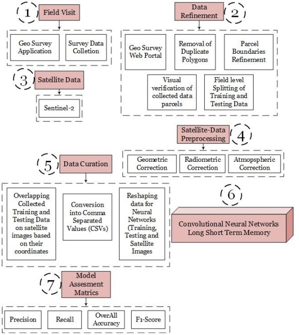
1. A brief overview of the modus operandi can be summarized in the following stages;

2. GTD is collected using the Geosurvey mobile application.

3. The data is split into training and testing with a 70/30 split ratio.

4. A synergy of Sentinel-2 and Planet-Scope is created to extract pixel information.

5. Temporal data of Sentinel-2 and Planet-Scope is taken for crop classification.

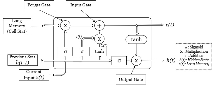
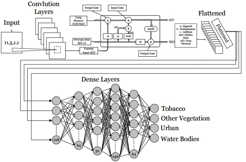
6. DLM-based ConvLSTM (A type of RNN) is developed.

7. During model training accuracy metrics are employed for measuring the performance of ConvLSTM.

8. The trained model is used for crop map generation.

9. The generated crop map consists of Tobacco plantation with a testing accuracy of 96.2%

10. Ground truth validation survey is also performed in the region of interest to ensure accurate classification results.

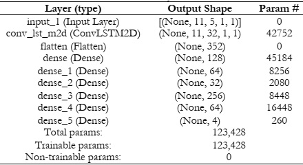
The summary or the formulation of the ConvLSTM model is given in Table .

Table 6: Model summary for ConvLSTM.

The methodology is implemented in our developed land cover land use system “Agriltytics” (Figure 10). More details about the system can be obtained from the website ncbcpeshawar.com.

Figure 10: A product derived from the conducted research.

Conclusion

Tobacco, a significant cash crop in the province of KP, is facing a growing challenge due to illicit cultivation, leading to substantial economic losses for the government due to tax evasion. The current methods used to estimate tobacco crop yields in the field rely on outdated measurement techniques. This research explores the application of advanced AI algorithms, specifically RNNs, to accurately identify tobacco crops. The study takes a collaborative approach, combining the capabilities of two prominent remote sensing satellite systems: the multispectral Sentinel-2 from the European Space Agency and Planet Scope by Planet Inc. Extensive surveys were conducted across four districts of KP over multiple tobacco growing seasons to collect GTD for obtaining necessary datasets required for training a neural network. Our developed RNN-based model, ConvLSTM, demonstrates positive results in the synergy of Sentinel-2 and Planet-Scope images, providing higher overall accuracy, as well as improved precision and recall scores for identifying tobacco plantations, compared to using Sentinel-2 alone. We believe that the implementation of the proposed approach on a larger scale can play a significant role in detecting illegal tobacco cultivation in the field, prompting timely action by government departments. Government should regulate policies for implementation of modern technologies for crop monitoring and acreage estimations and ensure funding and human resource development in these fields.

Figure 11: Classification map of area of interest (Dobian)

Acknowledgments:

The authors would like to express their gratitude to the survey team for their dedicated efforts in collecting ground truth data.

Author’s Contribution:

Original Draft, Waleed Khan; Conceptualization, Nasru Minallah; Formal Analysis, Atif Sardar Khan; Curation, Waleed Khan, Nasru Minallah, Atif Sardar Khan.

Conflict of Interest:

The authors declare no conflict of interest in publishing this manuscript in IJIST.

Reference

[1] R. T. Y. and R. Khalid, “Impact of tobacco generated income on Pakistan economy (a case study of khyber Pakhtunkhwa),” J. Basic Appl. Sci. Res., vol. 7, no. 4, pp. 1–17, 2017.

[2] and M. A. I. M. Sabir, W. Saleem, “Estimating the Under-Reporting of Cigarette Production in Pakistan,” 2022.

[3] W. K. et Al, “On the performance of temporal stacking and vegetation indices for detection and estimation of tobacco crop,” IEEE Access, vol. 8, pp. 103020–103033, 2020.

[4] and H. A. J. C. Antenucci, K. Brown, P. L. Croswell, M. J. Kevany, “Geographic Information Systems: a guide to the technology,” Springer, vol. 115, 1991.

[5] and P. J. P. Shanmugapriya, S. Rathika, T. Ramesh, “Applications of remote sensing in agriculture-A Review,” Int. J. Curr. Microbiol. Appl. Sci, vol. 8, no. 1, pp. 2270–2283, 2019.

[6] V. Klemas, “Fisheries applications of remote sensing: An overview,” Fish. Res., vol. 148, pp. 124–136, 2013.

[7] and G. A. D. Poli, F. Remondino, E. Angiuli, “Radiometric and geometric evaluation of GeoEye-1, World View-2 and Pléiades-1A stereo images for 3D information extraction,” ISPRS J. Photogramm. Remote Sens., pp. 35–47, 2015.

[8] M.-C. C. and C. Zhang, ““Formosat-2 for international societal benefits,” Remote Sens., pp. 1–7, 2016.

[9] M. Drusch et al., “Sentinel-2: ESA’s Optical High-Resolution Mission for GMES Operational Services,” Remote Sens. Environ., vol. 120, pp. 25–36, May 2012, doi: 10.1016/J.RSE.2011.11.026.

[10] C. San Francisco, “Planet application program interface: In space for life on Earth,” Team, P., 2017.

[11] C. Liao et al, “Synergistic use of multi-temporal RADARSAT-2 and VENμS data for crop classification based on 1D convolutional neural network,” Remote Sens., vol. 12, no. 5, 2020.

[12] and Y. H. J. Zhang, Y. He, L. Yuan, P. Liu, X. Zhou, “Machine learning-based spectral library for crop classification and status monitoring,” Agronomy, vol. 9, no. 9, 2019.

[13] G. B. and E. Scornet, “A random forest guided tour,” vol. 25, pp. 197–227, 2016.

[14] C.-C. C. and C.-J. Lin, “LIBSVM: a library for support vector machines,” ACM Trans. Intell. Syst. Technol., vol. 2, no. 3, pp. 1–27, 2011.

[15] and H. K. X. Sun, J. Peng, Y. Shen, “Tobacco plant detection in RGB aerial images,” Agriculture, vol. 10, no. 3, 2020.

[16] and M. S.-S. Y. Palchowdhuri, R. Valcarce-Diñeiro, P. King, “Classification of multitemporal spectral indices for crop type mapping: a case study in Coalville, UK,” J. Agric. Sci., vol. 156, no. 1, pp. 24–36, 2018.

[17] and X. L. D. Li, Y. Ke, H. Gong, “Object-based urban tree species classification using bi-temporal WorldView-2 and WorldView-3 images,” Remote Sens., vol. 7, no. 12, pp. 16917–16937, 2015.

[18] J. R. Jensen, “Biophysical remote sensing,” Ann. Assoc. Am. Geogr., vol. 73, no. 1, pp. 111–132, 1983.

[19] L. P. V. et Al., “Forecasting corn yield at the farm level in Brazil based on the FAO-66 approach and soil-adjusted vegetation index (SAVI),” Agric. Water Manag., vol. 225, 2019.

[20] and V. D. A. K. Verma, P. K. Garg, K. Hari Prasad, “CLASSIFICATION OF LISS IV IMAGERY USING DECISION TREE METHODS.,”,” Int. Arch. Photogramm. Remote Sens. Spat. Inf. Sci., vol. 41, 2016.

[21] and E. D. G. Z. Fan, J. Lu, M. Gong, H. Xie, “Automatic tobacco plant detection in UAV images via deep neural networks,” IEEE J. Sel. Top. Appl. Earth Obs. Remote Sens., vol. 11, no. 3, pp. 876–887, 2018.

[22] Y. B. Y. LeCun, “Convolutional networks for images, speech, and time series,” Handb. brain theory neural networks, vol. 3361, no. 10, 1995.

[23] and F. H. L. Wang, J. Zhang, P. Liu, K.-K. R. Choo, “Spectral–spatial multi-featurebased deep learning for hyperspectral remote sensing image classification,” Soft Comput., vol. 21, pp. 213–221, 2017.

[24] X. Z. et Al., “Deep learning in remote sensing: a review december,” 2017.

[25] and A. S. N. Kussul, M. Lavreniuk, S. Skakun, “Deep learning classification of land cover and crop types using remote sensing data,” IEEE Geosci. Remote Sens. Lett., vol. 14, no. 5, pp. 778–782, 2017.

[26] and Y. D. S. Ji, C. Zhang, A. Xu, Y. Shi, “3D convolutional neural networks for crop classification with multi-temporal remote sensing images,” Remote Sens., vol. 10, no. 1, 2018.

[27] S. Hochreiter and J. Schmidhuber, “Long Short-Term Memory,” Neural Comput., vol. 9, no. 8, pp. 1735–1780, Nov. 1997, doi: 10.1162/NECO.1997.9.8.1735.

[28] and A. M. A. Graves, N. Jaitly, “Hybrid speech recognition with deep bidirectional LSTM,” 2013 IEEE Work. Autom. speech Recognit. understanding, IEEE, pp. 273–278, 2013.

[29] L. M. and L. C. Jain, “Recurrent neural networks: design and applications.,” CRC Press, 1999.

[30] M. Boden, “A guide to recurrent neural networks and backpropagation,” Dallas Proj., 2002.

[31] and F. S. T. M. Breuel, A. Ul-Hasan, M. A. Al-Azawi, “High-performance OCR for printed English and Fraktur using LSTM networks,” 2013 12th Int. Conf. Doc. Anal. recognition, IEEE, pp. 683–687, 2013.

[32] and J. Y. Z. Ding, R. Xia, J. Yu, X. Li, “Densely connected bidirectional lstm with applications to sentence classification,” CCF Int. Conf. Nat. Lang. Process. Chinese Comput. Springer, pp. 278–287, 2018.

[33] X. Z. Y. Chen, K. Zhong, J. Zhang, Q. Sun, “LSTM networks for mobile human activity recognition,” Proc. 2016 Int. Conf. Artif. Intell. Technol. Appl. Bangkok, Thail., pp. 24–25, 2016.

[34] S. K. and R. Casper, “Applications of convolution in image processing with MATLAB,” Univ. Washingt., pp. 1–20, 2013.

[35] and J. Z. Z. Li, F. Liu, W. Yang, S. Peng, “A survey of convolutional neural networks: analysis, applications, and prospects,” IEEE Trans. neural networks Learn. Syst., 2021

Research Article

International Journal of Innovations in Science & Technology