Precipitation Trend Near Century (2020-2040):
Throughout the Near Century Research (NCR), various statistical parameters were
calculated on a monthly basis, including the Mean, Variance, Standard Deviation, Kurtosis,
Skewness, Range, Total Rainfall, Minimum Rainfall, and Maximum Rainfall (as shown in Table
1). According to the collected data, the average monthly rainfall exhibited variations, ranging
from a minimum of 30.4mm in September to a maximum of 252.4 mm in March. During this
particular time period, spanning nearly a century, the highest recorded level of precipitation in
the month of April was 1054.9mm, while the lowest recorded level was in September, at 1.0mm.
The Coefficient of Variation (CV%) for monthly rainfall, which represents the relative
fluctuation of the data in relation to the mean, ranges from 57.2% to 122.4% on average. The coefficient of variance was found to be highest in the month of November and lowest in the
month of July. The research also indicates that a positive Skew value was observed for each
month of the year, indicating that the amount of rainfall at the end of each month surpasses the
amount of rainfall at the beginning of each month.
Table 1:Monthly precipitation statistics in near century (2020-2040)
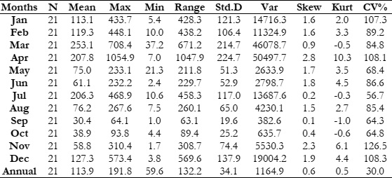
The coefficient of kurtosis exhibited its highest value of 10.3 during the month of April,
while the degree of skewness reached its lowest value of 0.1 in September. The calculated annual
standard deviation was found to be 34.1, while the monthly standard deviation varied between
19.6 and 224.7. Furthermore, it is evident that the annual precipitation pattern during the entire
duration of the study diverges from the customary distribution.
The winter and spring seasons, encompassing the months of December, January,
February, March, and April, exhibit the highest levels of monthly precipitation, characterized by
substantial rainfall. In contrast, the fall seasons, spanning September, October, and November,
experience minimal precipitation, often referred to as the harvesting season and a period of
aridity. According to the data presented in Table 1, the maximum annual rainfall recorded during
a span of 21 years is 191.8mm, while the smallest annual rainfall is 59.6mm.
Figure 2 illustrates the temporal variability of average annual precipitation data over a
span of nearly one hundred years. During the specified time frame, it is projected that the highest
recorded amount of rainfall will reach 191.8mm in the year 2035, while the lowest recorded
amount is anticipated to be 59.6mm in 2026.The data indicates a statistically insignificant upward
trend in precipitation levels within the region.
Temperature Trend Near Century (2020-2040):
Different statistical tests have been used to evaluate the trend in monthly data for the
near century analysis (2020-2040). The results have been calculated in Table 3 through
preliminary data analysis.
The greatest temperature recorded during this specific time frame is 16.5°C in the month
of June, while the minimum temperature is -6.0°C in January. The average monthly temperature
throughout the year varies between -3.1°C and 13.4°C, with the highest recorded in July and the
lowest in January. The annual standard deviation was determined to be 0.62, but the monthly
standard deviation varied between 1.10 and 2.10.
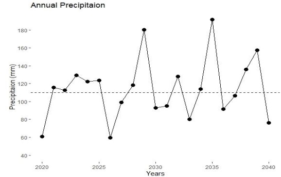
Figure
2:Annual precipitation trend for the period of near century (2020-2040)
Table 2:Monthly Mann-Kendall and Sen.’s slope results for precipitation in near century
(2020-2040)
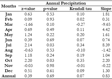
Table 3:Monthly Temperature statistics in near century (2020-2040)
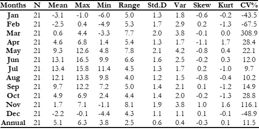
The region's yearly temperature shows uneven distribution, with positive and negative
skewness. It's left-skewed, with the highest CV in March (-67.5% to 308.9%) and the lowest in
February. Kurtosis ranged from -1.3 to 1.7: January, February, July, August, September,
October, and December have negative kurtosis (flat distribution), while others have positive
kurtosis (peaked distribution). See Table 3 for monthly and annual statistical values.
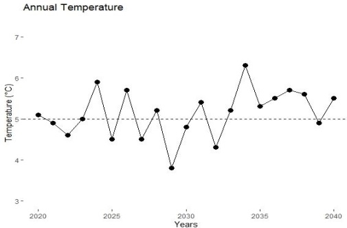
Figure
3:Annual Temperature trend for the period of near century (2020-2040)
Figure 3 illustrates the temporal variability of average yearly temperature data over a span
of nearly one hundred years. The projected highest mean temperature for the given time is
anticipated to reach 6.7°C in 2034, while the minimum is likely to be 3.8°C in 2029. The
temperature in the area exhibits a statistically insignificant upward trend over the specified time
period.
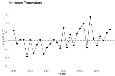
Figures 4 and 5 depict the trends in mean annual maximum temperature and lowest
temperature, respectively. Figure 4 exhibits a modest upward trend during the specified time
period. The mean maximum temperature exhibited fluctuations, ranging from 16.5°C in 2031
to 12.2°C in 2029. Figure 5 exhibits a pronounced upward trajectory that persists over the whole
duration under consideration. The mean lowest temperature exhibited fluctuations ranging from
-6.0°C in 2020 to -2.3°C in 2037.
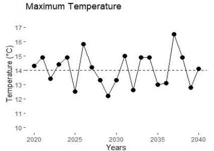
Figure
4:Annual Maximum Temperature trend for the period of near century (2020-2040)
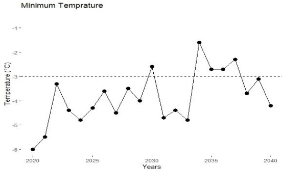
Figure
5:Annual Minimum Temperature trend for the period of near century (2020-2040)
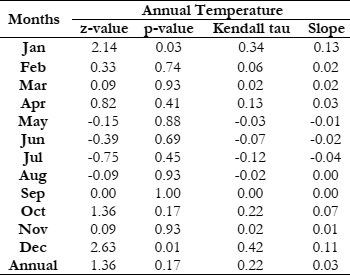
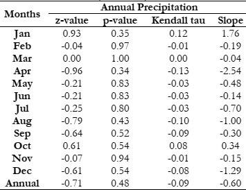
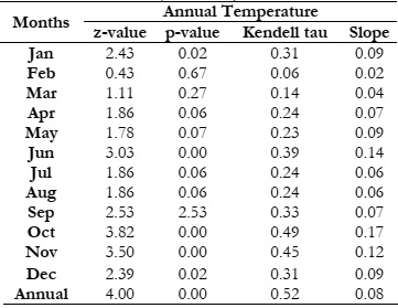
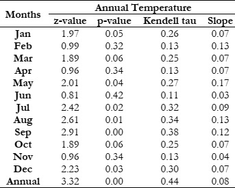
The MK and Sen's slope estimate methodologies were utilized at a monthly resolution
to examine the annual temperature data of the Jhelum Indus Basin, with the objective of
detecting any prevailing trends. The determination of the trend was performed using the least
significant level, which is the threshold at which the statistical significance of the trend is
established at the stated confidence level. The data shown in Table 4 demonstrates a lack of
statistical significance in the observed increase in annual temperature.
The p-values for the majority of the months indicate the presence of a discernible trend.
Positive Kendall tau values were seen during the study period in the months of January-April,
September- December. Negative Kendall tau values were seen in the months of May-August.
During the designated period of analysis, a broadly inconsequential positive trend was found in
the months of Jan-Apr, and Sep-Dec. Conversely, a generally inconsequential negative statistical
trend was identified in the months of May-Aug, with a confidence level of 95% (α = 0.05). The
majority of the month exhibits a positive slope value, indicating an increasing tendency.
Table 4:Monthly MK and Sen.’s slope results of temperature in near century (2020-2040)
Precipitation Trend Mid Century (2041-2070):
The Midcentury study analyzed monthly statistical parameters (Mean, Variance, SD,
Kurtosis, Skewness, Range, Total rainfall, Min-Max rainfall) shown in Table 5. Precipitation
varied monthly, from 31.9mm in September to 274.2mm in March. January had the highest (895.5mm) and September had the lowest (0.1mm) rainfall. Monthly rainfall's CV% ranged from
63.6% to 114.5%, highest in January and lowest in October. Positive Skew values indicated more
rainfall at month-end than at the beginning.
Table 5:Monthly precipitation statistics in midcentury (2041-2070)
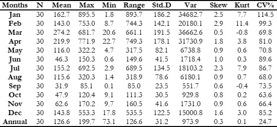
In February, kurtosis peaks at 11.4, and skewness is lowest at 0.5 in March. Annual SD
is 31.2; monthly SD ranges from 23.5 to 191.5. Summer, winter, and spring (Dec-May, Jul-Aug)
have high rainfall, while autumn (Sep-Nov) is dry. Table 5 shows max 199.7mm and min 73.1mm
annual rainfall in 30 years. Figure 6 depicts Midcentury's annual precipitation trends. Projections
indicate 199.7mm (2042) and 73.1mm (2055), showing a notable downward trend.
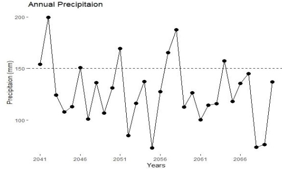
Figure
6:Annual precipitation trend for the period of midcentury (2041-2070)
Table 6 shows a significant decline in annual precipitation. Positive Kendall's tau
occurred in January, March, and October, but other months had negative values. January, March,
and October had a slight positive trend, while February to December exhibited a significant
negative trend (95% confidence). Most months displayed a declining tendency.
Table 6:Monthly Mann-Kendall and Sen.’s slope results of precipitation in midcentury (2041-2070)
Temperature Trend Mid Century (2041-2070):
In Table 7, the statistically significant variables, including standard deviation, average,
skewness, kurtosis, variance, range, and coefficient of variation, were calculated for the Monthly
temperature data spanning from 2041 to 2070 through preliminary data analysis. During this
period, the highest recorded temperature was 18.9°C in July, while the lowest recorded
temperature plummeted to -4.9°C in January. Across the year, the average monthly temperature
fluctuated between -1.9°C and 14.1°C. July witnessed the highest average temperature, whereas
February experienced the lowest. It is worth noting that the annual standard deviation remained
constant at 1.0, whereas the monthly standard deviation varied between 1.32 and 3.71.
Table 7:Monthly Temperature statistics in midcentury (2041-2070)
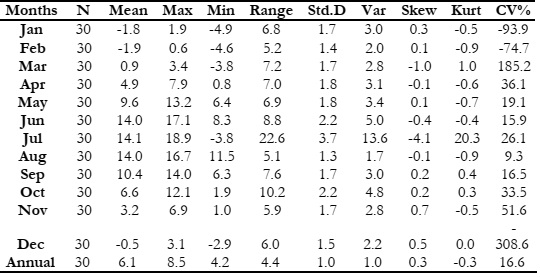
The region's annual temperature distribution showed both positive and negative
skewness, indicating unevenness. Monthly temperature CV ranged from -308.6% to 185.2%,
peaking in Mar and lowest in Dec. Kurtosis values ranged from -0.9 to 20.3: Jan-Feb, Apr-Aug,
and Nov had flat distributions, while other months were more peaked. Table 7 presents the
statistical parameters pertaining to both monthly and annual averages.
Figure 7 illustrates the variation in average yearly temperature data across the midcentury
era. The projected highest mean temperature for the year 2069 is anticipated to be 8.5°C, while
the minimum is likely to be 4.8°C in 2042. The temperature in the area exhibited a notable
upward trend throughout the specified time period.
Figures 8 and 9 depict the trends in mean annual maximum temperature and lowest
temperature, respectively. Figure 4.7 displays a notable upward trend during the specified time
period. The mean maximum temperature exhibited fluctuations, ranging from 18.9°C in 2069
to 12.8°C in 2043. Figure 9 illustrates a discernible upward trend over the specified time period. The mean lowest temperature exhibited fluctuations, ranging from -4.9°C in 2045 to -0.2°C in
2064.
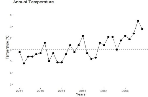
Figure
7:Annual Temperature trend for the period of midcentury (2041-2070)
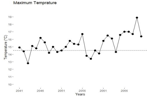
Figure
8:Annual Maximum Temperature trend for the period of midcentury (2041-2070)
Figure
9:Annual Minimum Temperature trend for the period of midcentury (2041-2070)
MK and Sen's slope methods were used to analyze Jhelum Indus Basin's annual
temperature data. Table 8 shows a significant upward trend in annual temperature. Positive
Kendall tau values in all months indicate a 95% confidence level for the upward trend. All
months display a positive slope, indicating an upward tendency.
Table 8:Monthly Mann-Kendall and Sen.’s slope results of temperature in midcentury (2041-2070)
Precipitation Trend End Century (2071-2099):
In the final century study, monthly rainfall data (Mean, Variance, SD, Kurtosis,
Skewness, Range) was analyzed (Table 9). Rainfall varied from 51.6mm (June) to 238.1mm
(March). March had the highest (840.3mm) and June the lowest (0.0mm) rainfall. CV% ranged
from 55.2% (June) to 110.2% (March). Positive Skew values indicated more end-of-month
rainfall.
Table 9:Monthly precipitation statistics in end century (2071-2099)
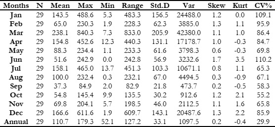
In December, kurtosis peaked at 2.2, while September had the lowest skewness at 0.2.
Annual SD was 33.1; monthly SD ranged from 21.8 to 205.9. Summer, winter, and spring had
intense rainfall, contrasting with minimal autumn precipitation (Sep-Nov). Table 9 shows max
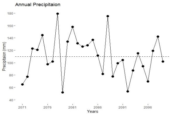
179.3mm and min 52.1mm annual rainfall in 29 years. Figure 10 depicts the variation in average
annual precipitation. A statistically negligible declining trend in the region's precipitation data
was observed.
Figure
10:Annual precipitation trend for the period of end century (2071-2099)
Monthly Mann-Kendall and Sen's slope analyses were done for annual rainfall in Jhelum
Indus Basin (Table 10). A statistically negligible decline in annual precipitation was observed.
Positive Kendall tau values were in May, June, Sep, Nov, Dec, while negative values were in Jan,
Feb, Mar, Apr, Jul, Aug, Oct. A slight positive trend was noted in May, Jun, Sep, Nov, Dec,
while Jan, Feb, Mar, Apr, Jul, Aug, Oct showed a significant negative trend (95% confidence).
Most months displayed a declining tendency.
Table 10:Monthly MK and Sen.’s slope results of precipitation in end century (2071-2099)
Temperature Trend End Century (2071-2099):
Table 11 presents statistically significant variables like standard deviation, average,
variance, skewness, range, coefficient of variation, and kurtosis for the monthly temperature
series from 2071-2099. In this period, July recorded the highest temperature at 20.9°C, while
January had the lowest at -6.1°C. Monthly average temperatures ranged from -0.7°C to 17.2°C,
with July being the warmest and February the coldest month. The annual SD was 1.2, while
monthly values varied from 1.4 to 2.9.
Table 11:Monthly Temperature statistics in end century (2071-2099)
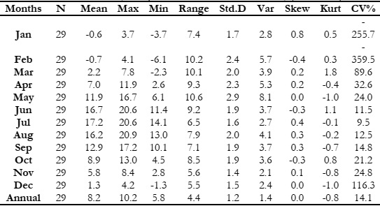
The annual temperature distribution exhibits both positive and negative skewness,
suggesting a lack of symmetry. The CV for monthly temperatures exhibited a range of -359.5%
to 116.3%, with the lowest value seen in February and the highest value observed in December.
The kurtosis values spanned from -1.0 to 1.8. Specifically, the months of April-August, and SepDec exhibited distributions that were relatively flat, as indicated in Table 11. Conversely, the
remaining months displayed distributions that were more peaked.
Figure 11 depicts the increasing trajectory observed in the average annual temperature
data throughout the last century. According to the projections, the anticipated maximum average
temperature is expected to reach 10.2°C by the year 2093, while the minimum average
temperature is estimated to be 5.8°C by 2076. The data presented in Figures 12 and 13 exhibit a
constant upward trajectory in the average annual maximum and minimum temperatures. The
observed values range from 15.1°C to 20.9°C for the mean annual maximum temperature, and
from -5.6°C to 3.1°C for the mean annual minimum temperature.
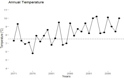
Figure
11:Annual Temperature trend for the period of end century (2071-2099)
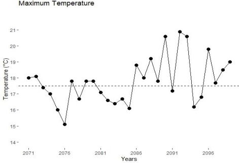
Figure
12:Annual Maximum Temperature trend for the period of end century (2071-2099)
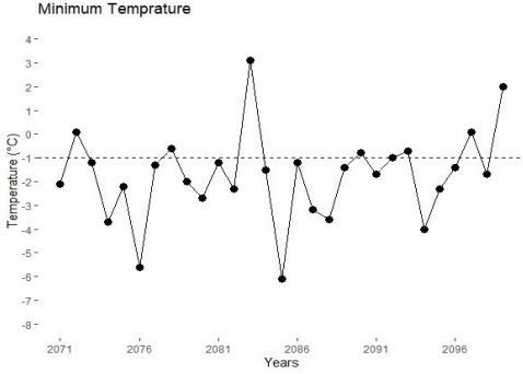
Figure 13:
Annual Minimum Temperature trend for the period of end century (2071-2099)
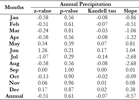
The MK and Sen's slope estimate approaches were employed on a monthly basis to
identify trends in the annual temperature data of the Jhelum Indus Basin. The estimation of the
trend was conducted by employing the least significant level, which denotes the threshold at
which the statistical significance of the trend is observed with a certain level of confidence. Table
12 exhibits a statistically significant upward trend in yearly temperature.
The p-values associated with the average months indicate the presence of a discernible
trend. Positive Kendall tau values were seen in all months during the study period. During the
designated period of analysis, a universally observed and statistically significant positive trend was seen across all months, with a confidence level of 95% (α = 0.05). All months exhibit a
positive slope value, indicating an upward tendency.
Table 12:Monthly MK and Sen.’s slope results of temperature in end century (2071-2099)
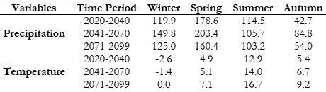
Seasonal Variation of Precipitation and Temperature for Future Period (2020-2099):
Table 13 displays the average values of precipitation and temperature for several seasonal
periods during future time intervals (2020-2040, 2041-2070, 2071-2099). Over the course of the
previous century, it was observed that spring had the most substantial amount of precipitation,
with a recorded average rainfall of 178.6mm. Conversely, autumn exhibited the lowest levels of
rainfall, with an average of 42.7mm. During the aforementioned period, the maximum
precipitation recorded during spring was 203.4mm, while the minimum precipitation observed
during autumn was 84.8mm. At the conclusion of the century, the spring season exhibited a
precipitation measurement of 160.4mm, while the autumn season observed a precipitation
measurement of 54.0mm. During the course of the investigation, it was observed that spring
had the greatest amount of precipitation, while autumn demonstrated the lowest levels. The data
indicates that there was a rise in precipitation towards the middle of the century, followed by a
subsequent fall towards the end of the century, so implying the occurrence of a peak in
precipitation during the mid-20th century.
In terms of temperature, it can be observed that the highest recorded average
temperature of 12.9°C was experienced during the summer season, while the lowest recorded
average temperature of -2.6°C occurred during the winter season throughout the course of the
past century. During the midcentury period, the average temperature during July was recorded
to be 14.0°C, while winter temperatures dropped to -1.4°C. By the conclusion of the century,
the average temperature of the summer season was recorded at 16.7°C, while the winter season
experienced temperatures as low as 0.0°C. Throughout all seasons, there was a noticeable
increase in temperatures throughout the midcentury in comparison to the preceding century,
with further escalation observed towards the conclusion of the century. In general, the data
indicates a consistent increase in temperatures over the duration of the research.
Table 13:Seasonal Variation of Precipitation and Temperature for Future Period (2020-2099)
Conclusion
This study analyzes temperature and precipitation data from 2020 to 2099. From 2020
to 2040, monthly precipitation varied (30.4mm in September to 253.1mm in March) and
temperatures fluctuated (-3.1°C in January to 13.4°C in July). There's a minimal upward trend
but not statistically significant. In the midcentury (2041-2070), March had the highest rainfall
(274.2mm), and September the lowest (31.9mm). There was a notable decrease in precipitation
and a corresponding temperature increase during this period. From 2071 to 2099, March had
the highest average rainfall, and June had the lowest. The basin exhibited a statistically significant
temperature increase over the final century. Precipitation patterns showed an upward tendency
in midcentury followed by a decline toward the end. Spring had the most rainfall, and autumn
had the least throughout the study periods. The examination of temporal fluctuations in rainfall
and temperature throughout prospective timeframes spanning from 2020 to 2099 unveils
intriguing patterns. The observed patterns indicate that there is an upward tendency in
precipitation levels throughout the midcentury era in comparison to the preceding near century,
followed by a subsequent decline in precipitation levels towards the conclusion of the century.
The data indicates a constant upward trend in temperature values from the early part of the
century to the middle, followed by a subsequent increase from the middle to the end of the
century. Furthermore, the data revealed that the highest amount of precipitation is experienced
during the spring season, whereas the lowest amount of rainfall is recorded during autumn
throughout all temporal intervals.
Abbreviations:
Intergovernmental Panel on
Climate Change (IPCC)
Hindu Kush Himalayas
(HKH)
Upper Indus Basin (UIB)
Hindu Kush Himalayas
(HKH)
Representative
Concentration Pathways
(RCPs)
Regional Climate Model
(RCM)
Million Acre-Feet (MAF)
Mann-Kendall (MK)
Jhelum River Basin (JRB)
World Meteorological
Organization (WMO)
Near Century Research
(NCR)
Coefficient of Variation (CV
%)
Standard Deviation (SD)
Reference
[1] M. DEMİRCAN, H. GÜRKAN, O. ESKİOĞLU, H. ARABACI, and M. COŞKUN,
“Climate Change Projections for Turkey: Three Models and Two Scenarios,” Turkish J.
Water Sci. Manag., vol. 1, no. 1, pp. 22–43, Jan. 2017, doi: 10.31807/TJWSM.297183.
[2] Z. P. Xu, Y. P. Li, G. H. Huang, S. G. Wang, and Y. R. Liu, “A multi-scenario ensemble
streamflow forecast method for Amu Darya River Basin under considering climate and
land-use changes,” J. Hydrol., vol. 598, p. 126276, Jul. 2021, doi:
10.1016/J.JHYDROL.2021.126276.
[3] H. Deng, Y. Chen, H. Wang, and S. Zhang, “Climate change with elevation and its
potential impact on water resources in the Tianshan Mountains, Central Asia,” Glob.
Planet. Change, vol. 135, pp. 28–37, Dec. 2015, doi:
10.1016/J.GLOPLACHA.2015.09.015.
[4] F. Giorgi and P. Lionello, “Climate change projections for the Mediterranean region,”
Glob. Planet. Change, vol. 63, no. 2–3, pp. 90–104, Sep. 2008, doi:
10.1016/J.GLOPLACHA.2007.09.005.
[5] H. Rodhe, “A comparison of the contribution of various gases to the greenhouse effect,”
Science, vol. 248, no. 4960, pp. 1217–1219, 1990, doi:
10.1126/SCIENCE.248.4960.1217.
[6] J. Stephenson, K. Newman, and S. Mayhew, “Population dynamics and climate change:
what are the links?,” J. Public Health (Bangkok)., vol. 32, no. 2, pp. 150–156, Jun. 2010,
doi: 10.1093/PUBMED/FDQ038.
[7] E. J. Kweka, E. E. Kimaro, and S. Munga, “Effect of deforestation and land use changes
on mosquito productivity and development in western kenya highlands: Implication for
malaria risk,” Front. Public Heal., vol. 4, no. OCT, p. 208939, Oct. 2016, doi:
10.3389/FPUBH.2016.00238/BIBTEX.
[8] multiple statistical downscaling methods over Pakistan’ [Atmospheric
Research 222 (2019) 114–133],” Atmos. Res., vol. 224, p. 196, Aug. 2019, doi: 10.1016/J.ATMOSRES.2019.03.030.
[9] T. Andrews et al., “Accounting for Changing Temperature Patterns Increases Historical
Estimates of Climate Sensitivity,” Geophys. Res. Lett., vol. 45, no. 16, pp. 8490–8499,
Aug. 2018, doi: 10.1029/2018GL078887.
[10] F. Nordio, A. Zanobetti, E. Colicino, I. Kloog, and J. Schwartz, “Changing patterns of
the temperature-mortality association by time and location in the US, and implications
for climate change,” Environ. Int., vol. 81, pp. 80–86, Aug. 2015, doi:
10.1016/J.ENVINT.2015.04.009.
[11] T. Ben-Gai, A. Bitan, A. Manes, P. Alpert, and S. Rubin, “Temporal and spatial trends
of temperature patterns in Israel,” Theor. Appl. Climatol., vol. 64, no. 3–4, pp. 163–177,
1999, doi: 10.1007/S007040050120/METRICS.
[12] C. Huntingford, P. D. Jones, V. N. Livina, T. M. Lenton, and P. M. Cox, “No increase
in global temperature variability despite changing regional patterns,” Nat. 2013 5007462,
vol. 500, no. 7462, pp. 327–330, Jul. 2013, doi: 10.1038/nature12310.
[13] J. M. Gregory and J. Oerlemans, “Simulated future sea-level rise due to glacier melt based
on regionally and seasonally resolved temperature changes,” Nat. 1998 3916666, vol.
391, no. 6666, pp. 474–476, Jan. 1998, doi: 10.1038/35119.
[14] A. A. Tahir, P. Chevallier, Y. Arnaud, L. Neppel, and B. Ahmad, “Modeling snowmeltrunoff under climate scenarios in the Hunza River basin, Karakoram Range, Northern
Pakistan,” J. Hydrol., vol. 409, no. 1–2, pp. 104–117, Oct. 2011, doi:
10.1016/J.JHYDROL.2011.08.035.
[15] M. Hassan, P. Du, R. Mahmood, S. Jia, and W. Iqbal, “Streamflow response to projected
climate changes in the Northwestern Upper Indus Basin based on regional climate
model (RegCM4.3) simulation,” J. Hydro-environment Res., vol. 27, pp. 32–49, Dec.
2019, doi: 10.1016/J.JHER.2019.08.002.
[16] A. F. Lutz, W. W. Immerzeel, P. D. A. Kraaijenbrink, A. B. Shrestha, and M. F. P.
Bierkens, “Climate Change Impacts on the Upper Indus Hydrology: Sources, Shifts and
Extremes,” PLoS One, vol. 11, no. 11, p. e0165630, Nov. 2016, doi:
10.1371/JOURNAL.PONE.0165630.
[17] A. J. Khan, M. Koch, and A. A. Tahir, “Impacts of Climate Change on the Water
Availability, Seasonality and Extremes in the Upper Indus Basin (UIB),” Sustain. 2020,
Vol. 12, Page 1283, vol. 12, no. 4, p. 1283, Feb. 2020, doi: 10.3390/SU12041283.
[18] A. A. Tahir, J. F. Adamowski, P. Chevallier, A. U. Haq, and S. Terzago, “Comparative
assessment of spatiotemporal snow cover changes and hydrological behavior of the
Gilgit, Astore and Hunza River basins (Hindukush–Karakoram–Himalaya region,
Pakistan),” Meteorol. Atmos. Phys., vol. 128, no. 6, pp. 793–811, Dec. 2016, doi:
10.1007/S00703-016-0440-6.
[19] A. F. Lutz, W. W. Immerzeel, A. B. Shrestha, and M. F. P. Bierkens, “Consistent increase
in High Asia’s runoff due to increasing glacier melt and precipitation,” Nat. Clim. Chang.
2014 47, vol. 4, no. 7, pp. 587–592, Jun. 2014, doi: 10.1038/nclimate2237.
[20] T. G. Andualem, D. A. Malede, and M. T. Ejigu, “Performance evaluation of integrated
multi-satellite retrieval for global precipitation measurement products over Gilgel Abay
watershed, Upper Blue Nile Basin, Ethiopia,” Model. Earth Syst. Environ., vol. 6, no. 3,
pp. 1853–1861, Sep. 2020, doi: 10.1007/S40808-020-00795-W/METRICS.
[21] S. A. Diress and T. B. Bedada, “PRECIPITATION AND TEMPERATURE TREND
ANALYSIS BY MANN KENDALL TEST: THE CASE OF ADDIS ABABA
METHODOLOGICAL STATION, ADDIS ABABA, ETHIOPIA,” African J. L.
Policy Geospatial Sci., vol. 4, no. 4, pp. 517–526, Sep. 2021, doi:
10.22004/AG.ECON.334454.
[22] M. Rizwan et al., “Simulating future flood risks under climate change in the source region
of the Indus River,” J. Flood Risk Manag., vol. 16, no. 1, p. e12857, Mar. 2023, doi:
10.1111/JFR3.12857.
[23] D. R. Archer, N. Forsythe, H. J. Fowler, and S. M. Shah, “Indus basin water resources
sustainability Sustainability of water resources management in the Indus Basin under
changing climatic and socio economic conditions Indus basin water resources
sustainability,” Hydrol. Earth Syst. Sci. Discuss, vol. 7, pp. 1883–1912, 2010, Accessed:
Sep. 28, 2023. [Online]. Available: www.hydrol-earth-syst-scidiscuss.net/7/1883/2010/