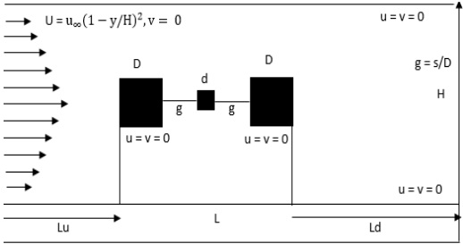
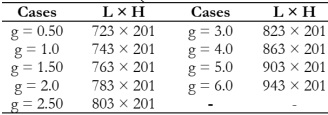
A 2-D numerical research is conducted to capture the flow behaviour when a small control rod is positioned between the two main rods. The range of g = 0.50 – 6.0 is used to determine the spacing between the main rods and control rod, while Re is selected between 80 and 200. Based on the analysis, the energy spectrum, vorticity contour, and physical properties are shown.
Vorticity Contour Visualization and Energy Spectrum:
We looked at six different flow modes in the situation of flow past two main rods with a tiny control rod positioned between the main rods at g = 0.50 – 6.0 and Re = 80 – 200 and named them based on their characteristics. At short gap spacings and relatively low Reynolds numbers (g = 0.50 – 1.50 at Re = 80 – 120), the first flow mode is generated. The existence of a control rod has no effect on the fluid flow in this flow mode. Figure 3(a–d) makes it evident how the fluid enters the channel and makes contact with the main rod C1. Without creating any flow between the gaps, the shear layer produced by C1 adhered to the control rod C2 as well as the main rod C2. Moreover, near the rear end of C2, the wake region lengthens as the Reynold number increases (see Figure 3v(a-d)). Vortex shedding did not occur throughout the computational zone as a result. This kind of flow is known as steady flow mode (SFM). There is no difference in lift or drag when vortex shedding is absent. No energy spectrum is produced as a result.
The shear layer detached from C1 in this flow mode and reattached to the in line control rod without creating vortices in the intervals between the breaks. As a result, vortices emerge at the rear end of C2, where the main rod experiences negative vertex shedding at its top surface and positive vortex shedding at its bottom surface. These vortices split off and start moving in different directions after a certain distance. The range of Re determines how many vortices form downstream of the computational domain; the higher the Reynolds number, the more vertices are formed and the shorter the wake zone. Figure 4 (a-c) provides a vivid illustration of this tendency.
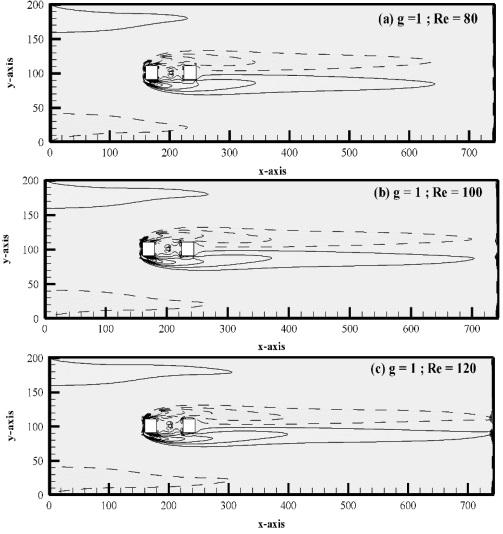
Figure 3: (a-d). Vorticity contour visualization for Steady Flow Mode.
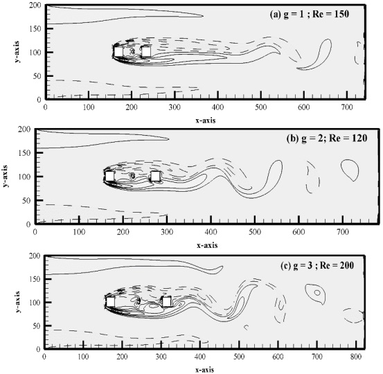
Figure 4: (a-c). Vorticity contour visualization for SLR Flow Mode
For both C1 and C2, the St graph shows a single peak when (Re, g) = (200, 0.50) is taken into account. However, the peak of C2 is broader than the peak of C1 due to a longer wake zone that emerges at C2's downstream location (see Figure 5(a)). However, as Figure 5(e) illustrates, multipeak are occasionally also seen for C2 as a result of both primary and secondary frequency.
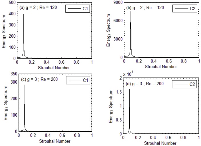
Figure 5: (a-d). Energy Spectrum analysis for SLR Flow Mode.
Currently, there are three flow modes in use: fully developed vortex shedding (FDVS). For Re = 80–160, it is examined at intermediate gap spacing, or g = 3.0 & 4.0. It is clear from Figure 6(a–d) that when there is enough gap separation between the main and control rods, vortices are also formed in the spaces between the gaps caused by the upstream, downstream, and control rods. There are two further classifications for this flow pattern: completely developed regular vortex shedding (i) and fully developed irregular vortex shedding (ii). As demonstrated in Figure 6(a, b), when fully developed normal vortex shedding takes place, vortices form between the gap and the downstream site of C2 and flow regularly towards the computational domain's exit without exhibiting disruptive behaviour. This flow characteristic is found at g = 3.0 and at Re Re = 80–120. Furthermore, behind the C2, a vor-karmann vortex-street forms. However, even if the vortices have fully formed in between the gaps, fully developed irregular vortex shedding shows vortex merging behaviour after reaching downstream of C2. These vortices move irregularly around the computational region. Figure 6(c,d) makes it clear that they are changing in size and strength. This flow mode happens at g = 3.0, at Re = 150 & 160.
C1 only exhibits one peak at (Re, g) = (150, 3.0) and (160, 3.0), but C2 exhibits numerous peaks. When it comes to C2, these various peaks are more noticeable when Re = 160 as opposed to 150. Additionally, it has been noted that when the Reynolds number rises, the value of St decreases.
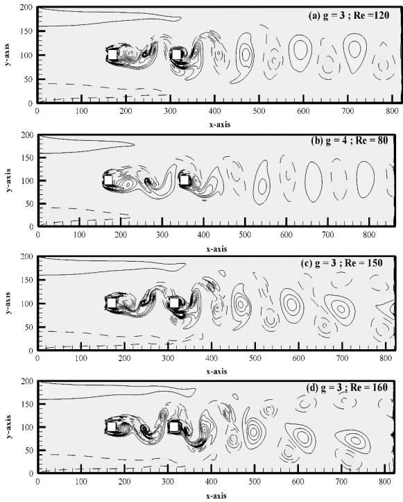
Figure 6: (a-d). Vorticity contour visualization for FDVS flow mode.
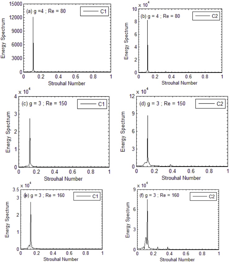
Figure 7: (a-f). Energy Spectrum analysis for FDVS Flow Mode.
An additional flow mode, FDTRVS, is shown in Figure 8(a-d). The vortices completely form within the gaps during this flow phase, however they form two rows downstream of the channel. Instead of moving in opposite directions towards the channel's outlet, positive and negative vortices move in parallel with one another. At Re = 100–200 for g = 4.0, Re = 80–175 for g = 5.0, and Re = 80–120 for g = 6.0, this flow phase was observed. Occasionally, tiny bubbles can be seen above and below the positive and negative vortex rows. It was named this mode. These bubbles cause the fully grown irregular two-row vortex to shed. The suitable energy spectrum, which has a single peak and no multiple peaks, is shown in Figure 9(a-d). For every scenario that was selected, the magnitude of St for C2 is higher than that of C1.
As shown in Figure 10(a, b), critical flow (CF) is seen at gap spacing 5.0 ≤ g ≤ 6.0 and Re from 160 to 200. The vortices in CF combine and deform among themselves after becoming fully developed downstream and within the gaps. The shed vortices are asymmetrical in size and shape and alter in strength as the Reynolds number rises. For every primary rod, the CF mode energy spectrum only reaches a single peak; however, for C2, as shown in Figure 11(a–d), the St peak is wider than it is for C1. All current flow modes for g = 0.50 – 6.0 and Re Re = 80 – 200 are shown in Table 4.
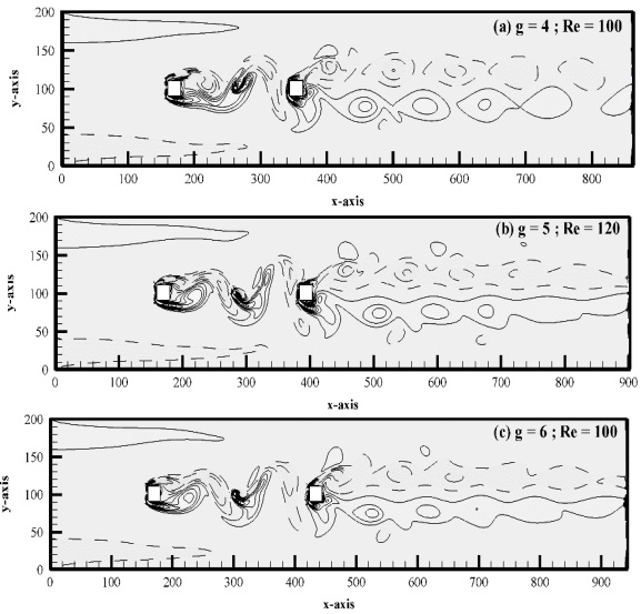
Figure 8: (a-c). Vorticity contour visualization for FDTRVS flow mode.
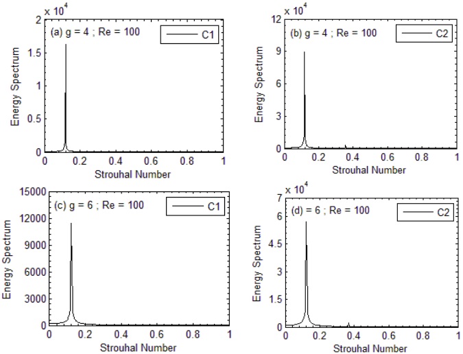
Figure 9: (a-d). Energy spectrum analysis for FDTRVS flow mode.
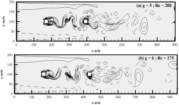
Figure 10: (a-b). Vorticity contour visualization for Critical flow mode.
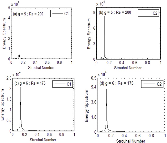
Figure 11: (a-d). Energy Spectrum analysis for Critical flow mode.
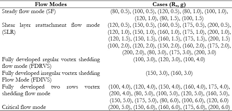
Table 4: All existing flow modes at g = 0.50 – 6.0 and Re = 80 – 200.
Effect of Gap Spacing and Reynolds Number on Physical Parameters:
Analyzing specific physical properties, such as Cdmean, Cdrms, Clrms, and St number, can help with the measurement of force fluctuation in fluid structure interaction problems. When g is kept above 3.0, the Cdmean of both rods exhibits increasing and declining behaviors. The SLR flow mode occurred at (Re, g) = (150, 3.0), when the Cdmean of C2 achieved its maximum value of 1.3907. The Cdmean of C2 started to climb at g = 3.0. Its lowest value was also discovered at (Re, g) = (200, 1.0). At (Re, g) = (200, 5.0), or 1.2609, the greatest value of Cdmean was obtained when the current flow mode was Critical (CF).
The drag coefficients (Cdrms) for both rods are displayed as root mean square values in Figure 12(c, d), and they demonstrate both increasing and decreasing behaviour as the Reynolds number rises. For particular Reynolds number values, Cdrms2 was observed to have the biggest magnitude when compared to Cdrms1. The location of the FDTRVS flow mode, (Re, g) = (160, 4), or 0.5168, is where the highest value of Cdrms2 is examined. Despite this, Cdrms1 peaks at (Re, g) = (160, 4.0), or 0.3570. Using the Steady flow SF mode, Cdrms2 and Cdrms1 both reached their lowest value at (Re, g) = (80, 0.5). These are, in order, 0.00003 and 0.00004.
The highest Clrms for C1 are 0.4365 at (Re, g) = (200, 4.0) and the lowest are 0.0000014 at (Re, g) = (80, 1.0). The SLR flow mode is formed at (Re, g) = (150, 3.0), where the maximum value of Clrms for C2 is 1.0303. Moreover, the root mean square values of C1 and C2 are larger than those of a single rod, with the exception of a negligible number of Clrms1 values at Re = 80.
Figure 12(g, h) plots the energy spectrum analysis against Reynolds number. The single rod statistics (g, h) are also shown in Figure 12 for comparison. While the values of St for C1 increase between Re = 80 and 150 before remaining constant for g = 1.0, 1.5, 4.0, and 5.0, the values of St for St1 expand between Re = 80 and 200 for g = 0.5. A mixed pattern is observed for g = 2.0, 3.0, and 6.0 for both C1 and C2, indicating that St1 and St2 behave in an increasing and then decreasing manner initially. In the case of C1, the St is less than the SC. The CF mode occurs at Re = 150–175 for g = 5.0–6.0, and St1 reaches its highest value of 0.1338 at that point. The greatest value of St for C2 is found to be 0.13411 at g = 6.0 and Re = 150–175.
The percentage decline in Cdmean against Re for g = 0.5 – 6.0 is shown in Figure 13(a, b). It begins to rise at g = 0.50 to 2.0, when the percentage reduction increases from Re = 80 to 160; at g = 3.0 to 6.0, it shows a mixed trend with an increase in Re for rod C1. In the case of C2, the mean drag coefficient shows increasing and decreasing behaviour at g = 3.0 and 4.0, but drops from Re = 80 to 200 at g = 0.50 to 2.0 and g = 5.0 & 6.0. At (Re, g) = (200, 3.0), the largest percentage decline in C1 is 19.3%; at (Re, g) = (175, 5.0) and (175, 6.0), the smallest reduction is 2.0. The largest and lowest drops for rod C2 were at (Re, g) = (200, 1.5) and (120, 3.0), at 120.3% and 1.5%, respectively.
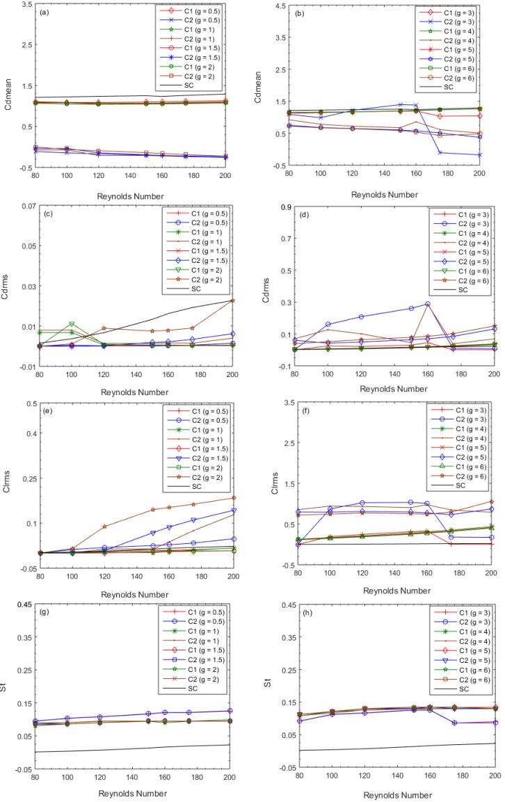
Figure 12: Variation of physical parameters, (a, b) Cdmean, (c, d) Cdrms, (e.f) Clrms and (g, h) St.
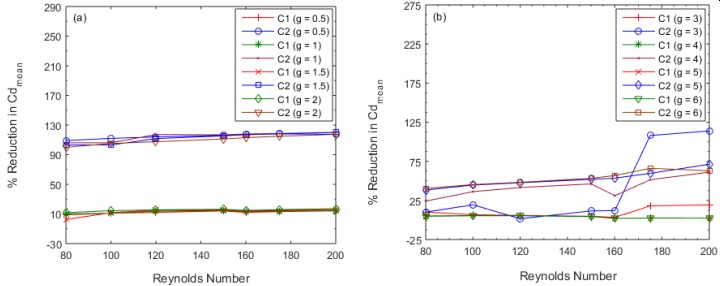
Figure 13: (a, b). Percentage reduction in values of Cdmean.
Conclusion
Examined are the effects of Re and g with Re = 80–200 and g = 0.50–6.0. The following are the primary conclusions of this study:
• The results of this study are utilized to investigate how changes in Re and g result in the acquisition of five distinct flow modes. * The critical flow mode, regular vortex shedding, irregular vortex shedding, two rows vortex shedding, and shear layer reattachment are all completely known flow modes. For any combination of (Re, g), it is noticed that the Cdmean of the C1 rod is bigger than the Cdmean of the C2 rod.Cdmean1 has the largest value at (Re, g) = (200, 5.0), or 1.2609, and Cdmean2 has the maximum value at (Re, g) = (150, 3.0), or 1.3907. * For g = 0.50 – 2.0 at Re = 80 – 200 and g = 3.0 at Re = 170 – 200, the Cdmean for C2 exhibits negative values.
• When the Reynolds number increases from Re = 80 to 200, the Cdrms and Clrms show different patterns.At (Re, g) = (200, 3.0), C1 has the most percentage reduction in Cdmean (19.3%); for C2, the biggest percentage reduction is 120.3% at (Re, g) = (200, 1.5) and (120, 3.0).
• The biggest value of St for C2 is studied at g = 6.0 for Re = 150 – 175, or 0.13411, while the maximum value of St1 is 0.1338 and occurs at Re = 150 – 175 for g = 5.0 – 6.0, while CF mode is occurring.
Nomenclature:
• C1 Upstream rod
• C2 Downstream rod
• Cs Speed of sound
• Cd1 Drag force of upstream rod
• Cd2 Drag force of downstream rod
• Cl1 Lift force of upstream rod
• Cl2 Lift force of downstream rod
• Cdmean1 Mean drag coefficients of upstream rod
• Cdmean2 Mean drag coefficients of downstream rod
• Cdrms Root-mean-square value of drag coefficients
• Clrms Root-mean-square value of lift coefficients
• D Diameter of the rod
• D Diameter of control rods
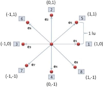
• ei velocity vectors
• Fd Force components in x- directions
• Fl Force components in y- directions
• hi Particle distribution function
• hi(eq) Equilibrium distribution function
• n Number of particles
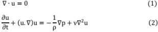
• p Pressure
• St Strouhal number
• U∞ Uniform inflow velocity
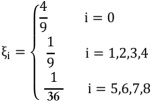
• ξi Weighting coefficient
Reference
[1] J. Y. Hwang and K. S. Yang, “Drag reduction on a circular cylinder using dual detached splitter plates,” J. Wind Eng. Ind. Aerodyn., vol. 95, no. 7, pp. 551–564, Jul. 2007, doi: 10.1016/J.JWEIA.2006.11.003.
[2] C. J. Doolan, “Flat-plate interaction with the near wake of a main rod,” AIAA S. J, vol. 47, pp. 475–478, 2009.
[3] S. Malekzadeh and A. Sohankar, “Reduction of fluid forces and heat transfer on a square cylinder in a laminar flow regime using a control plate,” Int. J. Heat Fluid Flow, vol. 34, pp. 15–27, Apr. 2012, doi: 10.1016/J.IJHEATFLUIDFLOW.2011.12.008.
[4] H. Sakamoto and H. Haniu, “Optimum Suppression of Fluid Forces Acting on a Circular Cylinder,” J. Fluids Eng., vol. 116, no. 2, pp. 221–227, Jun. 1994, doi: 10.1115/1.2910258.
[5] M. A. Z. Hasan and M. O. Budair, “Role of splitter plates in modifying cylinder wake flows,” https://doi.org/10.2514/3.12243, vol. 32, no. 10, pp. 1992–1998, May 2012, doi: 10.2514/3.12243.
[6] W. C. Park, “Numerical investigation of wake flow control by a splitter plate,” KSME Int. J., vol. 12, no. 1, pp. 123–131, 1998, doi: 10.1007/BF02946540/METRICS.
[7] C. Dalton, Y. Xu, and J. C. Owen, “THE SUPPRESSION OF LIFT ON A CIRCULAR CYLINDER DUE TO VORTEX SHEDDING AT MODERATE REYNOLDS NUMBERS,” J. Fluids Struct., vol. 15, no. 3–4, pp. 617–628, Apr. 2001, doi: 10.1006/JFLS.2000.0361.
[8] R. M. Darekar and S. J. Sherwin, “FLOW PAST A BLUFF BODY WITH A WAVY STAGNATION FACE,” J. Fluids Struct., vol. 15, no. 3–4, pp. 587–596, Apr. 2001, doi: 10.1006/JFLS.2000.0354.
[9] T. Tsutsui, T. & Igrashi, “Drag Reduction of a Circular rod in an Air-Stream,” J. Wind Eng. Ind. Aerodyn., vol. 4, no. 5, pp. 527–54, 2002.
[10] G. R. Vamsee, M. L. De Tena, and S. Tiwari, “Effect of arrangement of inline splitter plate on flow past square cylinder,” Prog. Comput. Fluid Dyn., vol. 14, no. 5, pp. 277–294, 2014, doi: 10.1504/PCFD.2014.064554.
[11] S. U. Islam, H. Rahman, W. S. Abbasi, and T. Shahina, “Lattice Boltzmann Study of Wake Structure and Force Statistics for Various Gap Spacings Between a Square Cylinder with a Detached Flat Plate,” Arab. J. Sci. Eng., vol. 40, no. 8, pp. 2169–2182, Aug. 2015, doi: 10.1007/S13369-015-1648-3/METRICS.
[12] R. Simenthy, V. Raghavan, and S. Tiwari, “Effect of Downstream Flapping Plate on the Flow Field Characteristics behind a Circular Cylinder,” no. 169.
[13] C. Y. Zhou, L. Wang, and W. Huang, “Numerical study of fluid force reduction on a circular cylinder using tripping rods,” J. Mech. Sci. Technol., vol. 21, no. 9, pp. 1425–1434, 2007, doi: 10.1007/BF03177429/METRICS.
[14] Q. D. Shao, C.P. & Wei, “Control of vortex shedding from a main rod,” AIAA J., vol. 46, pp. 397–407, 2008.
[15] C. H. Kuo and C. C. Chen, “Passive control of wake flow by two small control cylinders at Reynolds number 80,” J. Fluids Struct., vol. 25, no. 6, pp. 1021–1028, Aug. 2009, doi: 10.1016/J.JFLUIDSTRUCTS.2009.05.007.
[16] H. Wu, D. P. Sun, L. Lu, B. Teng, G. Q. Tang, and J. N. Song, “Experimental investigation on the suppression of vortex-induced vibration of long flexible riser by multiple control rods,” J. Fluids Struct., vol. 30, pp. 115–132, Apr. 2012, doi: 10.1016/J.JFLUIDSTRUCTS.2012.02.004.
[17] M. S. M. Ali, C. J. Doolan, and V. Wheatley, “Low Reynolds number flow over a square cylinder with a detached flat plate,” Int. J. Heat Fluid Flow, vol. 36, pp. 133–141, Aug. 2012, doi: 10.1016/J.IJHEATFLUIDFLOW.2012.03.011.
[18] A. Gupta and A. K. Saha, “Suppression of vortex shedding in flow around a square cylinder using control cylinder,” Eur. J. Mech. - B/Fluids, vol. 76, pp. 276–291, Jul. 2019, doi: 10.1016/J.EUROMECHFLU.2019.03.006.
[19] R. S. Serson, D., Meneghini, J.R., Carmo, B.S., Volpe, E. V. & Gioria, “Wake transition in the flow around a circular rod with a splitter plate,” J. Fluid Mech, vol. 755, pp. 582–602, 2014.
[20] L. Lu et al., “Numerical investigation of fluid flow past circular cylinder with multiple control rods at low Reynolds number,” J. Fluids Struct., vol. 48, pp. 235–259, Jul. 2014, doi: 10.1016/J.JFLUIDSTRUCTS.2014.03.006.
[21] S. U. Islam, H. Rahman, W. S. Abbasi, U. Noreen, and A. Khan, “Suppression of fluid force on flow past a square cylinder with a detached flat plate at low Reynolds number for various spacing ratios,” J. Mech. Sci. Technol., vol. 28, no. 12, pp. 4969–4978, Dec. 2014, doi: 10.1007/S12206-014-1118-Y/METRICS.
[22] S. U. Islam, R. Manzoor, Z. U. Islam, S. Kalsoom, and Z. C. Ying, “A computational study of drag reduction and vortex shedding suppression of flow past a square cylinder in presence of small control cylinders,” AIP Adv., vol. 7, no. 4, Apr. 2017, doi: 10.1063/1.4982696/22101.
[23] S. U. Islam, R. Manzoor, and C. Y. Zhou, “Effect of Reynolds Numbers on Flow Past a Square Cylinder in Presence of Multiple Control Cylinders at Various Gap Spacings,” Arab. J. Sci. Eng., vol. 42, no. 3, pp. 1049–1064, Mar. 2017, doi: 10.1007/S13369-016-2302-4/METRICS.
[24] D. T. Sukop, M. C. & Thorne, “Lattice Boltzmann modeling: an introduction for scientists and Engineers,” Springer Berlin Heidelb., 2005.
[25] D. A. Wolf-Gladrow, “Lattice-gas cellular automata,” pp. 39–138, 2000, doi: 10.1007/978-3-540-46586-7_3.
[26] T. G. Chapman, S., Cowling, “Mathematical Theory of Non-Uniform Gases,” Cambridge Univ. Press. Third Ed., 1970.