E-ISSN:2709-6130
P-ISSN:2618-1630

Research Article

International Journal of Innovations in Science & Technology

2023 Volume 5 Number 4 Oct-Dec

Remote Sensing-Based Prospectivity Maps Generation for Exploration of Minerals in Pakistan Using Machine Learning Techniques

Ehsin. S, Khan. W, Minallah. N

University of Engineering and Technology Peshawar

Abstract
The objective of this study is to generate and compare prospectivity maps that show the presence of Limestone in a specific area using remotely sensed data and machine learning techniques, in order to determine the most precise map that accurately depicts the presence of Limestone in that area. Remotely sensed data often utilize machine learning techniques to identify mineral formations and map geological features. Furthermore, machine learning techniques can also be used to generate prospectivity maps for mineral exploration. In this study, we utilized band ratios and principle component analysis (PCA) in conjunction with machine learning techniques to effectively identify Limestone formations and generate prospectivity maps for Limestone exploration using satellite imagery. Support Vector Machines (SVM) and Neural Networks (NN) were the machine learning techniques utilized on multispectral imagery from Sentinel-2 and Landsat-8. To assess the accuracy of the identification, the confusion matrix and kappa coefficient were employed. It was determined that the accuracy of the Neural Networks (NN) techniques was significantly better than the accuracy of the Support Vector Machines (SVM) techniques. The Neural Networks (NN) achieved an accuracy of 94.92% with a kappa value of 0.929, whereas the Support Vector Machine (SVM) had a maximum accuracy of 88.39% with a kappa value of 0.845. These high levels of accuracy and kappa coefficient values suggest that these machine techniques hold great potential for geological mapping and mineral exploration. The generated prospectivity maps can assist geologists and mining companies in identifying areas with a high potential for Limestone exploration, thereby reducing exploration costs and time.

Keywords: Machine Learning, Remote Sensing, Minerals, Multispectral, Prospectivity Maps.

Corresponding Author How to Cite this Article
Suleman Ehsin, University of Engineering and Technology Peshawar
Suleman Ehsin, Waleed Khan, Dr. Nasru Minallah, Remote Sensing-Based Prospectivity Maps Generation for Exploration of Minerals in Pakistan Using Machine Learning Techniques. IJIST. 2023 ;5(4):677-693 https://journal.50sea.com/index.php/IJIST/article/view/576

Introduction

Remote sensing is a revolutionary technology. It has changed the way we observe and understand the Earth remotely. Remote sensing has a wide spectrum of applications one of which is to detect and map various types of minerals, including metallic minerals such as gold, copper, iron, carbonate (Limestone, dolomite, gypsum), and non-metallic minerals such as phosphate, gypsum, and salt. Similarly, machine learning is an effective method for deriving conclusions from data and addressing complicated issues in a variety of fields, such as computer vision, natural language processing, recommendation systems, and predictive analytics. The availability of remote sensing data that encompasses multi and hyper-spectral capabilities, providing extensive resolutions in spatial, spectral, and temporal domains, together with recent advancements in image processing, have made remote sensing a powerful tool for geological research. Along with other geological uses, remote sensing has the capability to detect a range of minerals, including metallic minerals such as gold, copper, and iron, carbonate/calcite minerals like Limestone, dolomite, and gypsum, and non-metallic ones like phosphate, gypsum, and salt. Calcite minerals are highly valuable economically and exhibit unique reflection/absorption signatures [1]. Absorption features exhibited by carbonate minerals, including calcite, gypsum, and dolomite are in the range of 2.1-2.5 micrometers, and their reflectance typically occurs in the range of 1.55-1.75 micrometers in the SWIR region. These characteristics match closely with the characteristics of multispectral Landsat-8 imagery bands, specifically bands 7 (2.11-2.29μm) and 6 (1.57-1.65μm), as well as Sentinel-2 bands 12 (2.100–2.280 μm) and 11 (1.565–1.655 μm). Landsat-8 is widely recognized for its enhanced spectral and spatial characteristics in identifying mineral deposits and mineral exploration applications [2].

The utilization of band ratios and principal component analysis (PCA) methodologies are used to process and enhance the features of remotely sensed data [3][4]. Band ratio combinations are potential image processing methods for identifying different lithologies and effective methods for lithological discrimination. Additionally, it aids in minimizing illumination. The shadowing effect is very eminent in hilly areas which can also be reduced using band ratios [5][6].

For minimizing the number of image bands /dimensions and producing a color composite image for mapping hydroxyl-bearing Principal Component Analysis (PCA) is utilized [7]. Moreover, the use of band ratios (12/8, 2/5, (2+11+6)/ (3+4), and (4+6)/ (7+8)), and the PCA method with Sentinel-2A data has proven to be successful in identifying and distinguishing between various rock types in complex terrains [8]. The use of band ratios and PCA combined with machine learning algorithms can be an effective approach for accurately detecting different mineral formations from satellite imagery [9]. The RF model was able to generate better results than other models e.g., SVM and ANN and generated a prospectivity map indicating areas with high, medium, and low potential.

In order to distinguish between various subclasses of Limestone multispectral remote sensing data was evaluated, using different machine learning algorithms including naïve Bayes (NB), random forest (RF), classification, and regression tree (CART), and support vector machine (SVM) [10]. The RF algorithm achieved the highest accuracy of 96.36% compared to others. To evaluate which machine learning approach is more effective for locating carbonate outcrops in Landsat-8 data. The ANN MLP approach led with an F1 score of 0.823 while SVM and Random Forest (RF) had F1 scores of 0.810 and 0.812, respectively [11].

Similarly, the supervised classification approach has enhanced the lithological map of southern Morocco's Souk Arbaa Sahel area. Support vector machines (SVM) and ANN were used to process data, and the efficiency of both approaches was evaluated [12]. It was found that 85% of the formations were correctly classified including Limestone with SVM. In terms of classification accuracy, the SVM technique was found to perform better than artificial neural networks (ANN) [13].

This study will focus on carbonate exploration, particularly Limestone from multispectral satellite imagery of Landsat-8 and Sentinel-2 using Band ratio (BR), Principle Component Analysis (PCA) in combination with Support Vector Machine (SVM), and Neural Networks (NN), machine learning techniques.

Objectives:

To generate Prospectivity maps that indicate the presence of Limestone in a particular area using different satellites and different machine learning techniques and comparison of results(maps) that best fit the problem at hand. This study will assist geologists and mining companies in identifying areas with high mineral potential. It will also reduce their exploration cost and exploration time.

Novelty Statement:

In the domain of mineral mapping researchers have done a lot of work in the exploration of various minerals such as copper and gold (Au), in conjunction with the application of diverse machine learning models, including Support Vector Machines (SVM), Neural Networks (NN), Random Forest (RF), and Convolutional Neural Networks (CNN ) [14][15][16][17][18] but no significant literature is available targeting Limestone for perspectivity mapping. In this study, we are targeting Limestone to generate its prospectivity maps using different machine learning techniques and compare the techniques in order to find the technique with better accuracy. Additionally, we are not using traditional survey methods for data collection we are employing a Geo Survey application to collect data.

Material and Method

Study Area:

The study area falls in the territory of Mardan situated within Pakistan's Khyber Pakhtunkhwa province and is known for its rich mineral resources, including Limestone. Limestone is an important natural resource in the Mardan area and plays a significant role in the local economy. The area selected comes under the umbrella of 34°23'02.1"N, 72°07'27.1"E, as shown in Figure 1. A complete detail of the methodology is shown in Figure 2.

Figure 1: Generalized Location of Study Area on Map

Data Acquisition:

Remote sensing multispectral data acquisition is the process of collecting data from remote sensing platforms, such as satellites, aircraft, drones, etc., using sensors that capture information in multiple spectral bands. We will use multispectral data from the Landsat-8 satellite, sentinel-2 satellite, and ground data samples [19]. Table 1 shows the acquisition details of both the satellites.

Table 1: Acquisition details of satellite Images

Figure 2: Methodology Flow Diagram

Ground Survey for Data Collection:

Training data is very necessary while developing a robust machine learning model for remote sensing multispectral data. To collect Limestone training samples Geo Survey App was utilized. Geo survey app is designed and developed by the National Center of Big Data and Cloud Computing to help surveyors/scientists/researchers collect data using their smartphones [20]. Figure 3 provides a visual overview of the application, with Fig 3(a) showing the main menu having several survey methods. By tapping the desired method in the main menu, a polygon/polyline can be drawn around the survey area, as illustrated in Fig.3(b)(c)(d). The application was programmed using JAVA language and saved the survey data in Google’s database. Google’s database then provides data in JSON format which is then further converted into KML using Python language. ENVI was employed to convert the KML into shapefiles for testing and training the proposed technique’s/Model's performance.

Figure 3: (a) Main menu of application (b) Polygon drawn by tapping (c) View of survey data on map (d) List view of collected data

Data Processing:

Data processing involves the extraction of useful information by manipulation and analysis of data acquired from remote sensing instruments. The multispectral data processing is divided into the following steps:

Spatial Resampling:

Resampling is commonly performed in order to adjust the spatial resolution of satellite images. Depending on the specific requirements of the analysis or application either increase or decrease the spatial resolution of the image. In this study, we have increased image resolution, by using Bi-linear interpolation, as it creates new pixel values based on the weighted average of the surrounding pixels in a 2x2 neighborhood.

Layer Stacking:

Layer stacking creates a single image with multiple bands from multiple satellite images or raster layers. Each band in the stacked image represents a different spectral band or data layer from the original images. In this study, we have stacked the required bands from Landsat-8 and Sentinel-2 images for our analysis. Sentinel-2 data information is confined in a distinct spectral band which is 13 in number, similarly, Landsat-8 data information is loaded in 11 of its distinct spectral bands. Spectral bands were chosen while taking into account the depth, relevance, and extent of information they present. Keeping in view our study targets only 10 bands from Sentinel-2 were selected with a resolution of 10-20m and 7 bands of Landsat-8 were chosen with a resolution of 30m [21].

Temporal Stacking:

The process of temporal stacking involves aligning the images or raster layers, adjusting their spatial resolution, and assigning each layer to a separate band in the final stacked image. This allows analysts to visualize and analyze temporal changes in the landscape or the environment. Sentinel-2 and Landsat-8 images are temporarily stacked for this study. The resultant temporal stacked image (Composite Image) consists of a total of 17 bands of which 8 bands are from Lansat-8, and the remaining 9 are from Sentinel-2 [22].

Enhancement and Analysis:

The image enhancement techniques improve the visual quality of the data. The most common techniques for image enhancement are Principle Component Analysis (PCA) and Band Ratios, while for image analysis machine learning models are used.

Data Splitting:

A field survey of the proposed area was conducted to gather the samples using the Geo Survey Application. The samples were then segregated into a training dataset and a testing dataset having percentages of 70% and 30%.

Selection of Model:

Support Vector machines and Neural Networks are the two well-known machine learning algorithms/models that we have employed [23].

Support Vector Machines (SVMs):

Figure 4: Classification Using SVM

Figure 5: Simple Output Function of Neural Network with Weighted Inputs

Support Vector Machines (SVMs) fall into the category of supervised machine learning, known for solving the complex problems of regression and classification. SVM separates data into different categories using the best hyper-plane in a high-dimensional space [24]. The hyper-plane is chosen such that it maximizes the distance between the classes, which is known as the margin. In binary classification, two classes are separated by margins, their distance is further maximized to generate the hyper-plane shown in Figure 3. The same is the case with multiclass classification, multiple classes are separated by margins, and their distance is further maximized to generate a hyperplane shown in Figure 4. This hyperplane can be linear or non-linear, depending on the kernel used [25][26].

Once the SVM Model is trained, it has the capability to label the new unlabeled data into different classes. The SVM model maps the new data points into the same feature space as the training data and then predicts the class label. Handling high-dimensional data, non-linearly separable data, and avoiding overfitting are the few key features SVM offers over other machine learning techniques [27].

Neural Network:

A neural network Model is a complex machine-learning model designed after observing keenly the functional structure of the human brain [28]. Neural networks learn from the patterns found in data and then apply this learning to deal with real word problems e.g. image classification and pattern recognition, natural language processing, and predictive analytics [29].

Neural network architecture is divided into layers with interconnected neurons, the building block of a neural network. The neurons in the input layer receive training/testing data, and each subsequent layer hierarchically processes the data, extracting higher-level features as the data passes through the network. The output layer generates the output which can be a prediction, classification, or pattern based on the data fed into the input layer.

Each neuron performs its predefined computation as it receives inputs and then passes on to the next neurons in the next layer, where it is combined with the outputs of other neurons to produce a new set of outputs. Each neuron is assigned a weight which further helps in the interconnection of neurons. These weights can be adjusted, to minimize the error between the predicted output and the actual output, accordingly. During the training phase labeled data is fed into the input layer and weights are adjusted to achieve the maximum accuracy [30].

Neural networks have several different types, each has its own architecture and area of application. Feed-forward neural networks are considered the simplest, having a single layer of neurons that takes the input data and supplies output accordingly as shown in Figure 6. Neural networks are preferred over traditional machine learning models because of their complex nonlinear learning ability, which helps handle large datasets.

Model Evaluation:

The model is evaluated using the test data. Furthermore, the metrics that are used for model evaluation are overall accuracy, user accuracy, and producer accuracy [31]. The value of these metrics helps us identify if any problem lies in model training or parameter tuning.

Classification performance has been evaluated using the following parameters.

Confusion Matrix:

To evaluate the performance of a machine learning model confusion matrix is used. A confusion matrix is a table that provides a detailed view of classification models [32]. It specifies the classes where the model has promised results and the classes with dismal results. The confusion matrix can be extended to calculate other evaluation metrics, such as overall accuracy, user accuracy, and producer accuracy.

Some commonly used metrics calculated based on the confusion matrix include Overall Accuracy: The proportion of properly identified observations, calculated as;

Figure 6: A Simple Feed-Forward Neural Network Architecture

User Accuracy:

It is a measure of the probability that a specific class on the map corresponds to the same class on the ground, it assesses how well a particular land cover class is correctly identified or classified by the algorithm. High user accuracy indicates a low rate of false positives or misclassifications. Calculated as;

Producer Accuracy:

It is a measure of the probability that a specific class on the ground is correctly classified on the map. It evaluates how well the model correctly detects and classifies a specific land cover type. A high producer's accuracy indicates a low rate of false negatives or omission errors. Calculated as;

Kappa Coefficient:

The kappa coefficient is a statistical tool used to evaluate the degree of concurrence between two raters or classifiers [33]. The kappa coefficient is calculated by comparing the observed degree of concurrence between two raters or classifiers with the expected degree of concurrence that would occur by chance. Its value varies from -1 to 1, as the value goes towards 1 the degree of concurrence increases, and as the value moves towards 0 the degree of agreement falls which can be called by chance. Negative values indicate that the level of agreement is worse than the chance agreement. The kappa coefficient value is calculated:

Where Po is the observed degree of concurrence between the two raters or classifiers. Pe is the expected degree of concurrence by chance. The expected level of agreement by chance is calculated as follows:

Where a1 to an and b1 to bn are the marginal totals of the contingency table (the total number of times each rater/classifier assigns each category),n is the sum of all the observations.

Training and Testing of Model:

Models (SVM, NN) were trained and tested using the ground samples collected via the Geo Survey App. The data was categorized into training and testing samples. Each Category has four classes namely Limestone, Urban, Barren, and Vegetation. Each class was indicated with different colors, red indicates the Limestone, blue indicates the urban, brown indicates the barren, and green indicates vegetation. After successful training of the model, we tested the model using test samples collected from the ground survey. Training and testing lead to the generation of prospectivity maps which show the detailed contribution of each class in the pilot region.

Result and Discussion

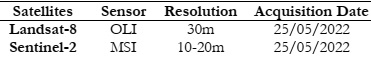
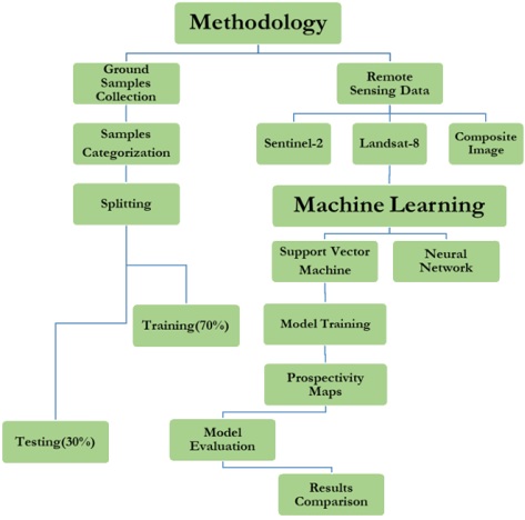
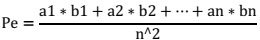
Prospectivity map generation techniques greatly assist geologists and mining companies in identifying areas with high mineral potential without physically visiting that area. It reduces their exploration cost and exploration. In this study, we have targeted the Limestone, a rich mineral resource found in Mardan, within Khyber Pakhtunkhwa province, Pakistan. We used different techniques to analyze this area while considering different datasets/imageries. Sentinel-2 and Landsat-8 data were considered for the prospectivity maps generation using machine learning models. Data was collected as different samples labeled into four classes namely Limestone, Urban, Barren, and Vegetation using the Geo Survey App. Data was trained and then tested using different machine-learning models with different kernel functions. After applying machine learning we came up with detailed maps showing the prospectivity of each class in that particular area. The detailed data of each model with its accuracy and kappa coefficient is shown in the tables below.

Band Ratios and Principle Component Analysis:

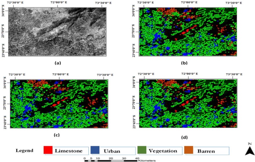
The results of different band ratios and PCA techniques highlight a certain area where there is a probability of the presence of Limestone. The different band composites using False Color Composite (FCC) are very helpful in lithological mapping. FCC of the ratio of 7/5, 6/4, and 4/2 band combinations are indicated in Figure 7(b). The plum color as highlighted shows an area that that has the possibility of the presence of Limestone. Similarly, the RGB of the ratio of 7/5, 3/2, and 4/5 band combinations is indicated in Figure 7(c). The pinkish color Limestone shows the possibility of the presence of Limestone [34].

In the same way, PCA is known for enhancing the image details adding more clarity, and highlighting the area that contains the Limestone. PC1, PC4, and PC3 are selected that contain more relevant information regarding carbonates [35]. PC1 has more bending towards carbonates. FCC of PC1, PC3, and PC4 was generated using RGB color composite and the result is displayed in Figure 7(d). In this analysis, the dark reddish area has the possibility of the presence of Limestone.

Support Vector Machine Analysis:

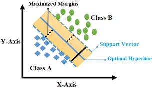
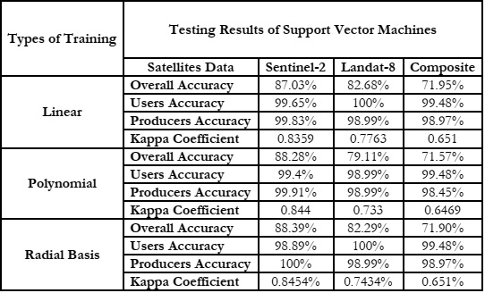
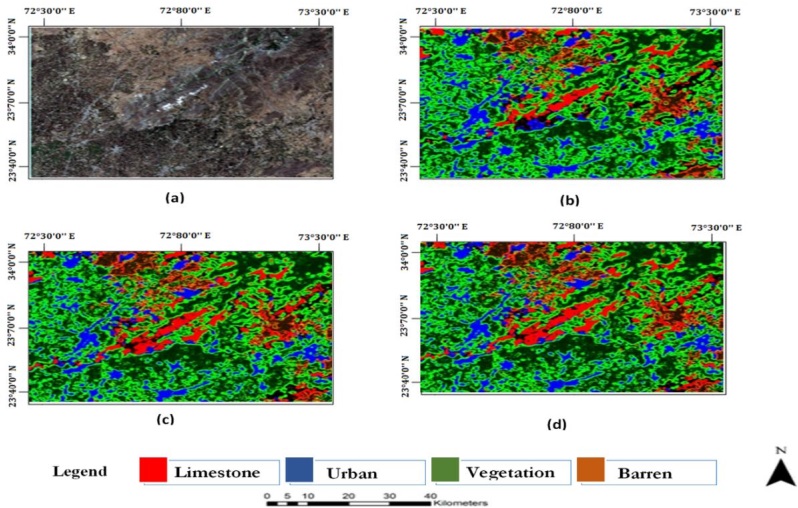
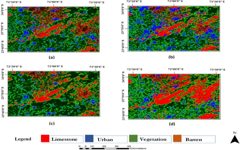
Remote sensing multispectral data is used to generate prospectivity maps, which identify areas that are likely to contain specific mineral or geological resources. After training the machine learning models on the prepared training data prospectivity maps are generated to highlight areas having the possibility to contain the Limestone. The Perspectivity maps against each technique using remotely sensed data are shown below in detail. In the maps below red area highlights the Limestone, blue highlights the Urban, green highlights the vegetation, and brown highlights the barren. The perspectivity map and accuracy of Sentinel-2 using SVM with different functions are shown in Figure 8 and Table 2. After testing SVM using different functions like linear, polynomial of degree 2, and radial basis, on the Sentinel-2 data, we have achieved the maximum accuracy of 88.38% using the radial basis function. SVM using different functions like linear, polynomial of degree 2, and radial basis on Landsat-8 data, also tested on Landsat-8, we have achieved the maximum accuracy of 80.57 using a linear function shown in Table 2. The prospectivity maps for the same are shown in Figure 9. The model is lagging accuracy when compared with the accuracy achieved in finding Limestone outcrop in the southwestern portion of the Potiguar Sedimentary Basin, Brazil [11]. The study was conducted using multispectral data from Landsat-8 employing machine models like MLP, SVM, and RF. The model was evaluated using the Confusion matrix and Mathews correlation coefficient (MCC). After proper training and testing of an SVM model, they achieved an accuracy of 91.87%. In the same way, SVM was applied on the Landsat-8 integrated with DEM of ALOS/PALSAR data for mapping Limestone at Souk Arbaa Sahel, Western Anti-Atlas, Morocco [12]. SVM with radial basis function was considered for this study because it carries good interpolation capabilities. An accuracy of 85% with a kappa value of 0.83 was achieved. It was also observed that our accuracy was leading when compared with another study conducted for the region, Bas Drâa inlier, Moroccan Anti Atlas. They used multispectral Landsat-8 data to map Limestone [36]. The model they selected was SVM. After proper training and testing of the model, they achieved an accuracy of 60.19% with kappa coefficients of 0.53. The detailed accuracy of each SVM function with its user and producer accuracy is shown in Table 2.

Figure 7: (a) Original Landsat-8 Image (b) FCC Image using band ratios 7/5,3/2, and 4/5 (c) FCC Image using band ratios 7/5, 6/4, and 4/2 (d) FCC Image Using PC1,PC4, and PC3

Table 2: Detailed training data of SVM model using Sentinel-2 data with its accuracy and kappa Coefficient

Neural Network Analysis:

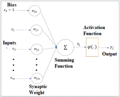
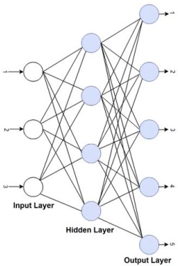
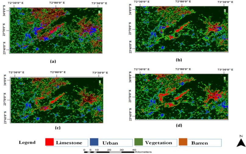
The same data, Landsat-8 and Sentinel-2, were then trained and tested using a Neural Network (NN) model on different iterations like 50,100,200,300. We have used the single hidden layer of NN for this analysis. After proper parameters tunning we achieved the maximum accuracy of 94.92% on 50 iterations which is shown in Table 3. The maps against each iteration were generated and shown in Figure 11 and Figure 12. The results of this technique are leading in terms of accuracy when compared with accuracy in finding Limestone outcrop in the southwestern portion of the Potiguar Sedimentary Basin in Brazil [11]. The study was conducted using multispectral data of Landsat-8 data employing machine models like MLP, SVM, and RF. The model was evaluated using the Confusion matrix and Mathew’s correlation coefficient (MCC). After proper training and testing of an MLP model, they achieved an accuracy of 92.14%. In the same way, NN was applied to the Landsat-8 data for mapping Limestone in Souk Arbaa Sahel Western Anti-Atlas, Morocco, the region [12]. The NN with a single layer was considered for training and testing and reached an accuracy of 68.40% with a Kappa coefficient of 0.65%, respectively.

Figure 8: (a)The Original Sentinel-2 Image (b) Perspectivity Map of Sentinel-2 Image Using SVM Linear Function (c) Perspectivity Map of Sentinel-2 Image Using SVM Polynomial Function (d) Perspectivity Map of Sentinel-2 Image Using SVM Radial Basis Function

Figure 9: (a) The Original Landsat-8 Image (b)Perspectivity Map of Landsat-8 Image Using SVM Linear Function (c) Perspectivity Map of Landsat-8 Image Using SVM Polynomial Function (d) Perspectivity Map of Landsat-8 Image Using SVM Radial Basis Function

Figure 10: (a)The Original Composite Image (b)Perspectivity Map of Composite Image Using SVM Linear Function (c)Perspectivity Map of Composite Image Using SVM Polynomial Function (d)Perspectivity Map of Composite Image Using SVM Radial Basis Function

The detailed accuracy of each iteration with its user’s and producer’s accuracy is shown in Table 3. From the above discussion, we could say that SVM itself is an effective model and has capabilities to predict and map different minerals remotely and NN is also known most complex problem-solving model in the domain of pattern recognition, pattern identification, and classification. But, the accuracy or the performance of a model varies with its area of application. The geography of the area greatly affects the model performance as we discussed earlier both models (SVM, NN) were tested for mapping Limestone using different areas/regions but the performance of the model was different on each pilot region. The accuracy/performance of a model also depends on the data on which the model was trained and tested. In the above discussion of SVM, we have tested the model for both Sentinel-2 and Landsat-8 data but SVM was performing well on Sentinel-2 data and an accuracy of 88.39% was achieved. Then, we changed the model from SVM to NN and tested the model for both Sentinel-2 and Landsat-8, it was performing well on Landsat-8 and gave the maximum accuracy of 94.92%. In the context of our study, we suggest that NN when trained on Landsat-8 data produces the best results.

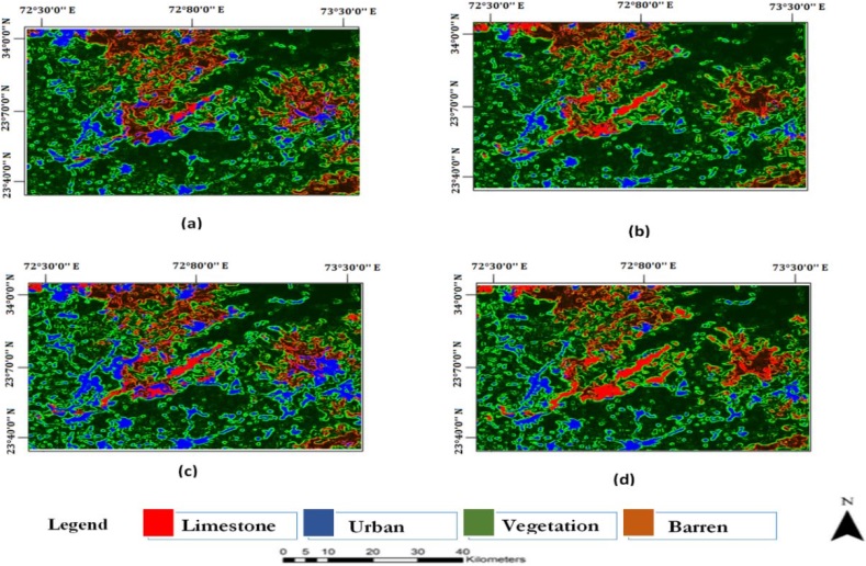
To study the behavior of these models we have generated another image by temporarily stacking Sentinel-2 and Landsat-8 data bands. The resultant temporal stacked image (Composite Image) consists of a total of 17 bands of which 8 bands were from Landsat-8, and the remaining 9 were from Sentinel-2. The composite image was then used to train the SVM and NN models. The perspectivity map and accuracy of Composite image data using SVM with different functions are shown in Table 2 and Table 3. The prospectivity maps of the same composite image were generated and shown in Figure 10 and Figure 13.

With SVM on Composite image data, we have achieved the maximum accuracy of 71.95% using a linear function, and with the same data when classified using a Neural Network (NN), we have reached the maximum accuracy of 92.64% on 50 iterations. The results of this Composite image data show that SVM is still not performing well on this composite image data, but NN is still leading in performance. Although the performance of NN on composite image data is less than the performance of Landsat-8 it's still much better than Sentinel-2's performance.

Table 3: Detailed testing data of SVM Model using Sentinel-2 Image with its accuracy and kappa Coefficient

Conclusion

In this paper, we have used remotely sensed data of Mardan region, a district of Khyber Pakhtunkhwa province of Pakistan for Limestone perspective map generation using machine learning techniques. Remotely sensed data from Landsat-8, and Sentinel-2 satellites were utilized for analysis and map generation. Field data was taken using the Geo Survey App. Supervised Machine learning models, SVM and NN were used for training and testing of satellite data, and finally, the results of both models were compared. Results showed that SVM with Radial Bias performs effectively on Sentinel-2 data for Limestone detection both visually and in terms of accuracy. An accuracy of 88.39% with a kappa coefficient of 0.85 was observed. User’s and producer’s accuracy also show a good contribution towards Limestone detection, 99.91%, and 98.89%. In the same way, the results of the Neural Network with 50 iterations perform actively on Landsat-8 data both visually and in terms of accuracy. An accuracy of 94.92% with a kappa coefficient of 0.9295 was observed. User’s and producer’s accuracy also shows a good contribution towards Limestone detection, 100, and 96.67.

So, in comparison to SVM and NN, NN outperforms SVM. The overall training and testing accuracy of satellite data is shown graphically in Figure 14. Additionally, band ratio and PCA are the two techniques utilized for detecting Limestone in the pilot area directly from satellite data. These techniques show good contribution towards Limestone detection and indicate the area that closely resembles the area indicated in maps generated by machine learning models. These techniques can further be applied to detect other minerals.

Figure 11: (a)Perspectivity Map of Sentinel-2 Image Using NN with 50 Iterations (b)Perspectivity Map of Sentinel-2 Image Using NN with 100 Iterations (c)Perspectivity Map of Sentinel-2 Image Using NN with 200 Iterations(d)Perspectivity Map of Sentinel-2 Image Using NN with 300 Iterations

Figure 12: (a)Perspectivity Map of Landsat-8 Image Using NN with 50 Iterations (b)Perspectivity Map of Landsat-8 Image Using NN with 100 Iterations (c)Perspectivity Map of Landsat-8 Image Using NN with 200 Iterations(d) Perspectivity Map of Landsat-8 Image Using NN with 300 Iterations

Figure 13: (a) Perspectivity Map of Composite Image Using NN with 50 Iterations (b) Perspectivity Map of Composite Image Using NN with 100 Iterations (c)Perspectivity Map of Composite Image Using NN with 200 Iterations (d)Perspectivity Map of Composite Image Using NN with 300 Iteration

Figure 14: Overall Training and Testing Accuracy Comparison Sentinel-2, Landsat-8, and Composite Image Classification

Future Work:

The field of remote sensing in minerals exploration is continually evolving, and several potential future directions and advancements can be anticipated. We can also extend the scope of this study in the following different ways; Advanced Remote Sensing Technologies as synthetic aperture radar (SAR) and unmanned aerial vehicles (UAVs), can be used to enhance the accuracy and resolution of Limestone detection and mapping. Advanced machine learning models e.g., Deep Learning can enhance the detection of Limestone deposits from remote sensing data by training models on annotated datasets to classify and map Limestone areas efficiently. 3D Modeling and Visualization utilizing remote sensing data, such as LiDAR, can create three-dimensional geological models of Limestone formations. This can aid in understanding the subsurface structure and potential mining implications. Mineral Mapping for Identification of specific minerals including Limestone formations can be enhanced using hyperspectral data. Hyperspectral data provides more insight into details about a particular area.

Reference

[1] J. L. Bishop et al., “Spectral Properties of Anhydrous Carbonates and Nitrates,” Earth Sp. Sci., vol. 8, no. 10, Oct. 2021, doi: 10.1029/2021EA001844.

[2] M. Sekandari et al., “Application of Landsat-8, Sentinel-2, ASTER and WorldView-3 Spectral Imagery for Exploration of Carbonate-Hosted Pb-Zn Deposits in the Central Iranian Terrane (CIT),” Remote Sens. 2020, Vol. 12, Page 1239, vol. 12, no. 8, p. 1239, Apr. 2020, doi: 10.3390/RS12081239.

[3] M. Greenacre, P. J. F. Groenen, T. Hastie, A. I. D’Enza, A. Markos, and E. Tuzhilina, “Principal component analysis,” Nat. Rev. Methods Prim. 2022 21, vol. 2, no. 1, pp. 1–21, Dec. 2022, doi: 10.1038/s43586-022-00184-w.

[4] Q. Ren, H. Zhang, D. Zhang, and X. Zhao, “Lithology identification using principal component analysis and particle swarm optimization fuzzy decision tree,” J. Pet. Sci. Eng., vol. 220, p. 111233, Jan. 2023, doi: 10.1016/J.PETROL.2022.111233.

[5] F. Abdelouhed, A. Algouti, A. Algouti, M. Ait Mlouk, and M. Ifkirne, “Lithological mapping using Landsat 8 Oli multispectral data in Boumalne, Imider, and Sidi Ali Oubork, High Central Atlas, Morocco,” E3S Web Conf., vol. 234, p. 00017, Feb. 2021, doi: 10.1051/E3SCONF/202123400017.

[6] N. Simon, C. Aziz Ali, K. Roslan Mohamed, and K. Sharir, “Best Band Ratio Combinations for the Lithological Discrimination of the Dayang Bunting and Tuba Islands, Langkawi, Malaysia,” Sains Malaysiana, vol. 45, no. 5, pp. 659–667, 2016.

[7] B. Mohammed, S. Hasan, and A. Mohsin Abdulazeez, “A Review of Principal Component Analysis Algorithm for Dimensionality Reduction,” J. Soft Comput. Data Min., vol. 2, no. 1, pp. 20–30, Apr. 2021, doi: 10.30880/jscdm.2021.02.01.003.

[8] M. H. Tangestani and S. Shayeganpour, “Mapping a lithologically complex terrain using Sentinel-2A data: a case study of Suriyan area, southwestern Iran,” Int. J. Remote Sens., vol. 41, no. 9, pp. 3558–3574, May 2020, doi: 10.1080/01431161.2019.1706203.

[9] T. Sun, F. Chen, L. Zhong, W. Liu, and Y. Wang, “GIS-based mineral prospectivity mapping using machine learning methods: A case study from Tongling ore district, eastern China,” Ore Geol. Rev., vol. 109, pp. 26–49, Jun. 2019, doi: 10.1016/J.OREGEOREV.2019.04.003.

[10] M. F. A. Khan, K. Muhammad, S. Bashir, S. U. Din, and M. Hanif, “Mapping Allochemical Limestone Formations in Hazara, Pakistan Using Google Cloud Architecture: Application of Machine-Learning Algorithms on Multispectral Data,” ISPRS Int. J. Geo-Information 2021, Vol. 10, Page 58, vol. 10, no. 2, p. 58, Feb. 2021, doi: 10.3390/IJGI10020058.

[11] V. Sales et al., “Analysis of Machine Learning Techniques for Carbonate Outcrop Image Classification in Landsat 8 Satellite Data,” Int. Geosci. Remote Sens. Symp., vol. 2022-July, pp. 3604–3607, 2022, doi: 10.1109/IGARSS46834.2022.9883577.

[12] I. Bachri, M. Hakdaoui, M. Raji, A. C. Teodoro, and A. Benbouziane, “Machine Learning Algorithms for Automatic Lithological Mapping Using Remote Sensing Data: A Case Study from Souk Arbaa Sahel, Sidi Ifni Inlier, Western Anti-Atlas, Morocco,” ISPRS Int. J. Geo-Information 2019, Vol. 8, Page 248, vol. 8, no. 6, p. 248, May 2019, doi: 10.3390/IJGI8060248.

[13] B. Es-Sabbar, A. Essalhi, M. Essalhi, and B. Karaoui, “Variscan structural evolution and metallogenic implications at the paleozoic maider basin, eastern anti-atlas, Morocco,” J. African Earth Sci., vol. 207, p. 105060, Nov. 2023, doi: 10.1016/J.JAFREARSCI.2023.105060.

[14] C. Zheng et al., “Mineral prospectivity mapping based on Support vector machine and Random Forest algorithm – A case study from Ashele copper–zinc deposit, Xinjiang, NW China,” Ore Geol. Rev., vol. 159, p. 105567, Aug. 2023, doi: 10.1016/J.OREGEOREV.2023.105567.

[15] M. Abedini, M. Ziaii, T. Timkin, and A. B. Pour, “Machine Learning (ML)-Based Copper Mineralization Prospectivity Mapping (MPM) Using Mining Geochemistry Method and Remote Sensing Satellite Data,” Remote Sens. 2023, Vol. 15, Page 3708, vol. 15, no. 15, p. 3708, Jul. 2023, doi: 10.3390/RS15153708.

[16] H. Li et al., “Convolutional neural network and transfer learning based mineral prospectivity modeling for geochemical exploration of Au mineralization within the Guandian–Zhangbaling area, Anhui Province, China,” Appl. Geochemistry, vol. 122, p. 104747, Nov. 2020, doi: 10.1016/J.APGEOCHEM.2020.104747.

[17] M. Yao, Z. Jiangnan, M. Yao, and Z. Jiangnan, “Advances in the application of machine learning methods in mineral prospectivity mapping,” Bull. Geol. Sci. Technol. 2021, Vol. 40, Issue 1, Pages 132-141, vol. 40, no. 1, pp. 132–141, doi: 10.19509/J.CNKI.DZKQ.2021.0108.

[18] K. Wang, X. Zheng, G. Wang, D. Liu, and N. Cui, “A Multi-Model Ensemble Approach for Gold Mineral Prospectivity Mapping: A Case Study on the Beishan Region, Western China,” Miner. 2020, Vol. 10, Page 1126, vol. 10, no. 12, p. 1126, Dec. 2020, doi: 10.3390/MIN10121126.

[19] M. E. D. Chaves, M. C. A. Picoli, and I. D. Sanches, “Recent Applications of Landsat 8/OLI and Sentinel-2/MSI for Land Use and Land Cover Mapping: A Systematic Review,” Remote Sens. 2020, Vol. 12, Page 3062, vol. 12, no. 18, p. 3062, Sep. 2020, doi: 10.3390/RS12183062.

[20] “Geo Survey - Land Survey - Apps on Google Play.” Accessed: Nov. 22, 2023. [Online]. Available: https://play.google.com/store/apps/details?id=com.ncbc.survey.gis&hl=en&gl=US&pli=1

[21] R. H. Topaloğlu and E. Sertel, “ASSESSMENT OF CLASSIFICATION ACCURACIES OF SENTINEL-2 AND LANDSAT-8 DATA FOR LAND COVER / USE MAPPING”, doi: 10.5194/isprsarchives-XLI-B8-1055-2016.

[22] W. Khan et al., “On the Performance of Temporal Stacking and Vegetation Indices for Detection and Estimation of Tobacco Crop,” IEEE Access, vol. 8, pp. 103020–103033, 2020, doi: 10.1109/ACCESS.2020.2998079.

[23] B. Mahesh, “Machine Learning Algorithms—A Review.,” International Journal of Science and Research. Accessed: Nov. 22, 2023. [Online]. Available: https://www.scirp.org/(S(i43dyn45te-exjx455qlt3d2q))/reference/referencespapers.aspx?referenceid=3168174

[24] T. T. Dai and Y. S. Dong, “Introduction of svm related theory and its application research,” Proc. - 2020 3rd Int. Conf. Adv. Electron. Mater. Comput. Softw. Eng. AEMCSE 2020, pp. 230–233, Apr. 2020, doi: 10.1109/AEMCSE50948.2020.00056.

[25] I. Roman, R. Santana, A. Mendiburu, and J. A. Lozano, “In-depth analysis of SVM kernel learning and its components,” Neural Comput. Appl., vol. 33, no. 12, pp. 6575–6594, Jun. 2021, doi: 10.1007/S00521-020-05419-Z/METRICS.

[26] L. Sunitha and M. B. Raju, “Multi-class classification for large datasets with optimized SVM by non-linear kernel function,” J. Phys. Conf. Ser., vol. 2089, no. 1, p. 012015, Nov. 2021, doi: 10.1088/1742-6596/2089/1/012015.

[27] S. Sharma, S. Srivastava, A. Kumar, and A. Dangi, “Multi-Class Sentiment Analysis Comparison Using Support Vector Machine (SVM) and BAGGING Technique-An Ensemble Method,” 2018 Int. Conf. Smart Comput. Electron. Enterp. ICSCEE 2018, Nov. 2018, doi: 10.1109/ICSCEE.2018.8538397.

[28] O. I. Abiodun, A. Jantan, A. E. Omolara, K. V. Dada, N. A. E. Mohamed, and H. Arshad, “State-of-the-art in artificial neural network applications: A survey,” Heliyon, vol. 4, no. 11, p. 938, Nov. 2018, doi: 10.1016/J.HELIYON.2018.E00938/ATTACHMENT/7F6968D1-2173-4A69-BC61-62AD41135D5C/MMC2.

[29] A.-N. Sharkawy, “Principle of Neural Network and Its Main Types: Review,” J. Adv. Appl. Comput. Math., vol. 7, pp. 8–19, Aug. 2020, doi: 10.15377/2409-5761.2020.07.2.

[30] S. Singu and S. Singu, “Comparative Analysis of Artificial Neural Networks,” Int. J. Mach. Learn. Sustain. Dev., vol. 3, no. 4, Dec. 2021, Accessed: Nov. 22, 2023. [Online]. Available: https://www.ijsdcs.com/index.php/IJMLSD/article/view/192

[31] A. Tharwat, “Classification assessment methods,” Appl. Comput. Informatics, vol. 17, no. 1, pp. 168–192, 2018, doi: 10.1016/J.ACI.2018.08.003/FULL/PDF.

[32] J. S. Y. K. F. F. Howard, C. B. Boye, I. Yakubu, “Image Classification and Accuracy Assessment Using the Confusion Matrix, Contingency Matrix, and Kappa Coefficient,” Int. J. Comput. Inf. Eng, vol. 17, no. 9, pp. 511–518, 2023.

[33] W. Tang, J. Hu, H. Zhang, P. Wu, and H. He, “Kappa coefficient: a popular measure of rater agreement,” Shanghai Arch. psychiatry, vol. 27, no. 1, pp. 62–67, 2015, doi: 10.11919/J.ISSN.1002-0829.215010.

[34] H. Ghrefat, A. Y. Kahal, K. Abdelrahman, H. J. Alfaifi, and S. Qaysi, “Utilization of multispectral landsat-8 remote sensing data for lithological mapping of southwestern Saudi Arabia,” J. King Saud Univ. - Sci., vol. 33, no. 4, p. 101414, Jun. 2021, doi: 10.1016/J.JKSUS.2021.101414.

[35] A. Ja’afar Abubakar, M. Hashim, and A. Beiranvand, “USING LANDSAT 8 (OLI) REMOTE SENSING DATA TO MAP LITHOLOGY AND MINERALOGY FOR GEOTHERMAL RESOURCE EXPLORATION”.

[36] “Lithological mapping using Landsat 8 OLI and Terra ASTER multispectral data in the Bas Drâa inlier, Moroccan Anti Atlas.” Accessed: Nov. 22, 2023. [Online]. Available: https://www.spiedigitallibrary.org/journals/journal-of-applied-remote-sensing/volume-10/issue-01/016005/Lithological-mapping-using-Landsat-8-OLI-and-Terra-ASTER-multispectral/10.1117/1.JRS.10.016005.full