Appraisal of Urban Heat Island over Gujranwala and its Environmental Impact Assessment using Satellite Imagery (1995-2016).

Syeda Areeba Gillani1, Saif-ul-Rehman2, Hafiz Haroon Ahmad1, Abdul Rehman1, Sarwar Ali1, Atif Ahmad1, Usama Junaid1, and Muhammad Zubair Atiq1.
1 Remote Sensing group, Department of Space Science, University of the Punjab, Quaid-e-Azam Campus, Lahore, Punjab, Pakistan.
2 Department of Geography, Government College University Lahore.
*Correspondence | Syeda Areeba Gillani E.Mail. syedaareebagillani@gmail
Citation | Gillani.S.A, Rehman.S, Ahmad.H.H, Rehman.A, Ali.S, Ahmad.A, Junaid.U, and Ateeq.Z Appraisal of Urban Heat Island over Gujranwala and its Environmental Impact Assessment using Satellite Imagery (1995-2016). International Journal of Innovations in Science and Technology, Vol 01 Issue 01: pp 1-14, 2019.
DOI | https://doi.org/10.33411/IJIST/2019010101
Received | Dec 14, 2018; Revised |Jan 24, 2019 Accepted | Jan 25, 2019; Published | Jan 28, 2019.
________________________________________________________________________
Abstract.

Rapid urbanization and concretization are the main sources of formation and existence of Urban Heat Island (UHI). Due to high concentration of pollutants in urban environments, the residents are exposed to unexpected health issues. This study aims at delineating the temporal variations in the spatial extent of UHI over Gujranwala using Landsat thermal imagery. It also aims at determining the variations in pollutant concentration in the atmosphere due to vehicle’s tailpipe emissions and fossil fuel burning by industrial plants. We used various indices e.g., NDVI, NDBI, NDWI and land surface temperature calculations to investigate spatiotemporal variations in urban growth patterns and their impacts on the UHI. The results show that the UHI enlarged in all direction specially in the north west during the study period which is similar to urban growth trends. There also exist positive correlation between industrial and vehicle’s discharge with pollutant’s concentration in atmosphere. Remote sensing tools proved elegant in trend mapping and analysis.
Keywords: Urban heat island, Normalized Difference Vegetation Index (NDVI), Normalized Difference Built-up Index (NDBI), Normalized Difference Water Index (NDWI), Land Surface Temperature (LST).
1. Introduction.
The recent migration trends of masses toward developed cities in search of basic needs of life is very common around the world. It is the main reason of extensive urbanization [1] which has transformed the metropolitan areas into heat islands [2]and this phenomenon is termed as Urban Heat Island (UHI) [3]. The speedy urbanization has enhanced the anthropogenic activities that have led to the development of urban microclimates. Microclimates are getting warmer due to many factors including tailpipe emissions by vehicles used for transportation, fossil fuel and coal burning by industrial plants and the cooking concentration at domestic and commercial level [1]. The growth of vehicles adds greenhouse gasses and Chloro Fluoro Carbons (CFCs) in the atmosphere which absorb the outgoing long wave radiations that contribute to increase the city temperature more than periphery. Urban heat islands are of two types: 1) Atmosphere heat island 2) Surface heat island. The atmospheric heat island is further subdivided in two types: 1) Urban canopy layer; and 2) Urban boundary layer.
The surface heat island can be studied in detail due to availability of freely available remotely sensed datasets [3]. These datasets have motivated researchers to investigate the main sources of urban heat reservoirs currently available worldwide [4].The urban heat can be analyzed by extracting the Land Surface Temperature (LST) through satellite derived data. A wide range of thermal datasets recorded by various sensors including Advanced Spaceborne Thermal Emission and reflection (ASTER), Advanced Very High Radiometer (AVHRR), Moderate Resolution Imaging Spectrometer (MODIS), Landsat 5 Thematic Mapper (TM), Landsat-7/Enhanced Thematic Mapper (ETM) and Landsat-8 (TIRS 1,2) are useful to extract the pixel-based surface temperature. Various researches have focused on the relationship of Land Use Land Cover (LULC) with LST [5],and found that the changes in LST are dependent upon the spatial arrangement of urban settlements.
The natural vegetation is the main source of carbon sinks which is removed to established new settlements [6, 7]. The negative impacts of new settlements are extensively studied to determine the influence of LULC on urban environment e.g. Ding et al., 2013 [8] investigated the relation of LULC with LST using Landsat images. Similarly, Jusuf et la., 2007 [9] used LST data to explore the consequence of LULC changes on the spatiotemporal pattern of UHI in Singapore. Zang et al. 2013 [10] evaluated the rate of increasing population on UHI patterns in Shanghai. Li et al., 2011 [11] computed LST and Normalized Difference Vegetation Index (NDVI) to understand the impacts of urban sprawl on the landscape of Shanghai. Kuang et al., 2015 [12] examined the difference of LST for different LULC classes and pointed out that urban areas were found warmer than vegetative areas. The thermal properties of land have been altered by modification in LUCL of an area that causes the change in energy budget, creating the UHI. Zhang 2008 [13] studied various urban factors including urban area, water body, vegetative area, and the mean NDVI to map the spatial extent of UHI. Singh 2004 [14] monitored the seasonal variations in LST of Dehli using Landsat TM data. NDVI is a common indicator used to discriminate the vegetation existing in an area from other features like built-up area and the water body [15]. Lo et al., 2003 [16] used NOAA-AVHRR data to compute temporal variations in NDVI and LST to map LULC changes in Iberia. Similar studies were conducted by Kawashina 1994 [17] for Tokyo, the pearl river delta China [18] , the Atlanta metropolitan area [15, 19, 20] through Landsat thermal datasets. Many other studies explored the relationship between LST, land surface emissivity and NDVI [21, 22, 23, 24]
The main objectives of this research were to delineate the temporal variations in the spatial extent of urban heat island over Gujranwala and to appraise the impacts of various pollutants involved in heat traps using satellite images from (1995-2016) in ARC GIS interface.
2. Materials and methods.
2.1 Investigation site.
Gujranwala is among the seven most populous areas in Pakistan. It is located in northeast of Punjab province in Pakistan. It is bordered by the districts including Sheikhupura in the south, Hafizabad, and Gujrat in west and Sialkot in the northeast. Gujranwala is known as a third largest industrial center after Karachi and Faisalabad in Pakistan that contributes to 5% in national Gross Domestic Product (GDP)(Gujranwala Wikipedia https://en.wikipedia.org/wiki/Gujranwala). It has hot and semi-arid climate where temperature ranges between 36 to 46 oC in summer and drops to 5 oC in winter. The spatial extent of Gujranwala is mapped in Figure 1.

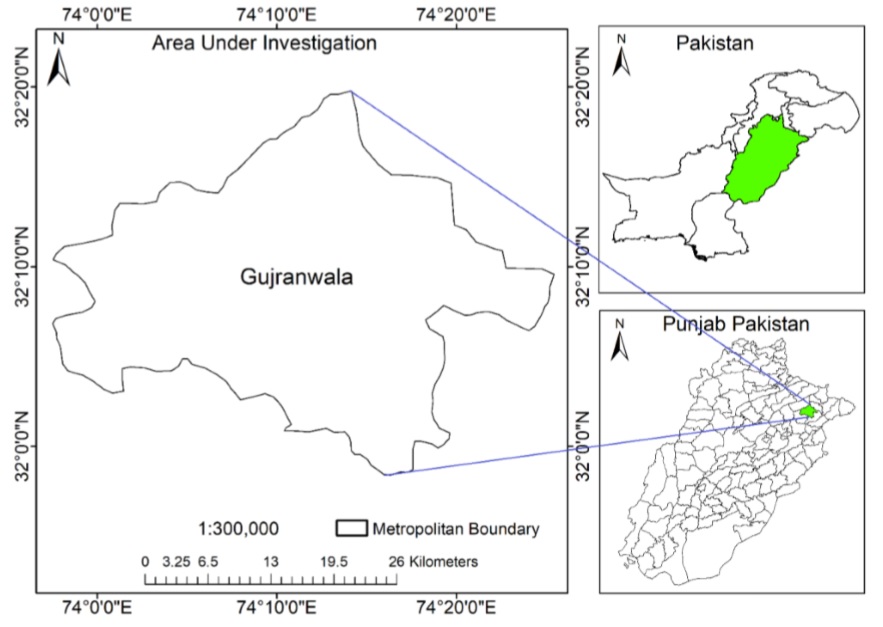
Figure 1. Study site.
2.2 Material and methods.
The spatiotemporal patterns of LST are explored and compared using various indices including NDVI, Normalized Difference Built-up Index (NDBI) and the
Normalized Difference Water Index (NDWI). The contemporary advantage of this research was to use remote sensing data in wider issues relating to the impacts of variations in NDVI and LST on the environment and human health. We used Landsat satellite imagery listed in Table 1, freely available on United State Geological Survey (USGS) website (https://earthexplorer.usgs.gov) to estimate the spatiotemporal variations in vegetation, built up and water indices. Thermal datasets are the valuable products of Landsat series that return pixel-based temperature values.
Table 1. Landsat image acquisition dates.

2.3 Pixel-based temperature calculation for Landsat 8 thermal bands.
Landsat 8 started functioning on April 10, 2013, with a wider range of spectral bands within visible, infrared and thermal wavelengths. Band 10 (B10) and Band 11 (B11) are known as thermal bands commonly used to compute pixel-based temperature values. A thermal dataset is comprised of an array of pixels and each pixel preserves a unique number called Digital No (DN). Initially, the DN values are converted to irradiance using Equation 1 as below, Irradiance = (3.342x10-4 x Thermal
band)+0.1 (1) The value 3.342x10-4 is mentioned in the metadata file (.MTL) saved by a complete Landsat image. Equation 1 is useful to extract pixel-based irradiance in (watt/m2srad). The irradiance-based dataset is further converted to temperature using the Equation 2 as below,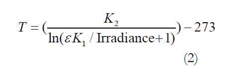

Where K1 and K2 are constants and their values are mentioned in the metadata file of each Landsat 8 image as below.
K1 for B10 = 774.89
K1 for B11 = 480.89
K2 for B10 = 1321.08
K2 for B11 = 1201.44
Where ε is emissivity and its value is taken as 0.95 [25]. The complete procedure of extraction of pixel-based temperature values is mentioned on USGS website.
(http://landsat.usgs. gov/Landsat8_Using_ Product.php).
2.4 Pixel based temperature calculation for Landsat 5,7 thermal bands.
Thematic Mapper (TM) in Landsat 5 and Enhanced Thematic Mapper Plus (ETM+) in Landsat 7 also offer thermal band B6. However, the procedure to analyze pixelbased temperature variations is quite similar for the both thermal bands produced by TM and ETM+ [26]. Initially, the DN values are converted to spectral radiance using the
Equation 3 as below,
Lλ= Lmin+ (Lmax- Lmin) x DN/255 (3)
Where Lλ is spectral radiance, Lminand Lmax are the variations in radiance. The values assigned to Lminand Lmaxare 607.7 and 1260.56 respectively. We used the Equation 4 to extract pixel based temperature values in centigrade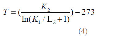

2.5 Calculation of built up, vegetation and water indices.
NDVI is a vegetation index commonly used to determine the spatial extent and health of vegetation in an area. It is widely used index that considers a spectral band within near infrared wavelength and the other in red wavelength using the Equation 5 below [4, 18, 20].

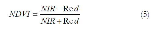
NDVI ranges between -1 to +1 where +1 highlights the vegetation and -1 represents all the feature other than vegetation. NDBI is commonly used index to map the built-up areas and barren lands. Built-up areas experience a drastic increase in reflectance in the Shortwave Infrared (SWIR) wavelength range (1.55-1.75)μm and are markedly lower in the Near Infrared (NIR) wavelength i.e., (0.76-0.90)μm. The
differentiation between these two wavelength ranges results in positive values
for built-up pixels [27] as follows, 

NDWI is the water index that is commonly used to enhance the reflectance of water bodies within a study site. The formula used to compute NDWI is as follows, 

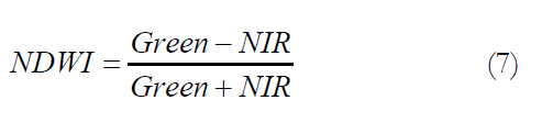
Water reflects maximum in green wavelength range (0.52-0.60)μm and absorbs all the heat radiations within NIR range.
2.6 Regression analysis.
Regression is a statistical indicator used to determine the strength of the relationship between two variables. We used regression to compute the relationship for spatiotemporal variations between concentrations of various pollutants in comparison to their sources.
2.7 GIOVANNI.
GIOVAANI is web-based forum sponsored by National Aeronautics and Space Administration (NASA) that provides spatiotemporal variations in concentration of atmospheric gases globally. We used GIOVANNI to extract the information about atmospheric constituents that play a vital role in increasing the LST by capturing the terrestrial heat.
Results and discussion.
We selected the satellite imagery for the months May and June to compute the vegetation indices e.g., NDVI, NDWI, and NDBI for the study site. During these months the study area receives maximum sunshine hours and peak solar flux which is important to delineate UHI. Also, we can get high contrast for the indices to map the extent of major features including built-up area, water body, and the vegetation. NDVI is an important indicator commonly used to map the spatial extent of vegetation existing in an area. We used Equation (5) to generate NDVI based datasets for all satellite images mentioned in Table 1 using spectral bands in NIR and red wavelength ranges and mapped the results in Figure (2) A1-A5, where the lush green areas are vegetation and the red regions are non-vegetative features. NDBI is an elegant indicator that highlights the built-up features including buildings, road networks and open areas etc. This index is used to distinguish urban areas in comparison to other features like vegetation or water body. We used Equation (6) to generate NDBI based datasets for all Landsat images mentioned in Table (1) using the spectral bands in SWIR and NIR wavelength ranges and mapped the results in Figure (2) (B1-B5). NDWI is an index which is used to make prominent the water body existing in a dataset. Water is a good absorber of heat in infrared wavelength that reflects nothing toward satellite’s sensor, therefore, we get waterbody in blackish tone in a remotely sensed dataset hence water area is difficult to demarcate properly. NDWI is used as a substitute to delineate water features existing in an area. We applied Equation (7) to all the datasets mentioned in Table 1 to delineate the water body and mapped results in Figure 2 (C1-C5).
Temperature effects the human activities and consumption of biomass of an area. Various crop promoting activities to achieve targeted productivity level is operated by temperature. These activities include 1) the impact assessment of net radiations on plant growth 2) the effects of elevated temperature on biomass generation and 3) the effects of heat stress on the water intake capacity by plants, therefore, it is important to manage the temperature range which is considered optimum for the proper growth of a particular plant.
The heat generation in an area is largely dependent upon various factors including the existing land use, number of vehicles, industrial emissions, and burning of fuels. The temperature of the study site is increasing every year that needs to be monitored to create a balance between the urban area in comparison to its surroundings. We computed pixel-based temperature datasets using thermal bands for all satellite images mentioned in Table 1 and mapped the results in Figure 2 (E1 to E5). We extracted vegetation from all NDVI based datasets, built-up areas from NDBI datasets, water from NDWI based datasets and made composites by taking their integrated impact e.g., the composite made for the year 1995 consisted of the collective impact of three indices using raster calculator utility in Arc GIS 10.1. This method of generation of composites is comparatively accurate as per other methods of feature mapping using classification utility. We used Equations (1,2) for thermal datasets of Landsat 8 and the Equations (3,4) for Landsat 5,7 to compute pixel-based temperature values.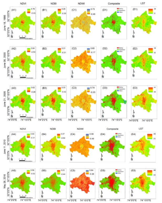

Figure 2. Spatiotemporal variations in NDVI, NDBI, NDWI and LST (oC).
Spatiotemporal variations mapped in Figure 2 determine that the total area under investigation was 861 km2. This area was partitioned by three dominating features including built-up area, water body, and the vegetation. The maps (A1 to A5) in Figure 2 are showing a decline to the vegetative area of 725 km2was under vegetation in the year 1995 that degraded to320 km2 in 2016. Whereas the maps (B1 to B5) in Figure 2 describes progressive jumps to built-up area. Built up area was estimated as 93 km2 in 1995 that increased up to 318 km2 in 2016. Built-up area was observed with a remarkable boost of 78 km2 during 2010 to 2016. The maps (C1 to C5) in Figure2 highlights the water body which seems with no change in area under water flow. The water area was observed as43 km2 in 1995 that remained unchanged in 2016. We observed a slight increase in water area in the map C4 in Figure 2 which was the accumulation of rainfall water that removed after some days by evaporation and seepage by the earth. The composites containing an amalgam of all existing features were mapped (D1 to D5) in Figure 2 which show a degradation to vegetation in comparison to built-up areas. Spatiotemporal variations in land use patterns (D1 to D5) were analyzed that determine the temporal shift of built-up areas toward north-west direction at large scale and a reasonable sprawl in all directions at small scale. Maps (E1 to E5) in Figure 2 determines the spatial variability of lands surface temperature. The comparison of maps (D1 to D5) with (E1 to E5) in Figure 2 shows the same trend for hotspots marked with red color which means that the spatial extent of heat islands is highly dependent on built-up land use patterns, e.g., the shape of heat island in map E1 was centralized according to the built-up extent mapped in D1 that show similar patterns for heat island as per temporal changes in built-up land use.
2.8 Effects of atmospheric gasses on urban heat islands.
The concentration of various gases e.g., (CO2, CO, NO2, and SO2) plays a vital role in increasing the atmospheric temperature. These gases are capable enough to capture longwave radiations emitted by the surface of earth creating a natural greenhouse effect. The impacts of these gasses cannot be ignored while investigating the UHI phenomenon in an industrial region like Gujranwala therefore, we collected temporal variability of these gasses from GIOVANNI for our study area and analyzed the main sources of production of air pollutants in term of CO2, CO, NO2 and SO2. These pollutants are highly involved in blockage of urban heat and the terrestrial radiations which cause to make the urban areas as heat islands. There are many sources which produce these pollutants but there are two major sources including the fuel burning by the vehicles and the industrial emissions. These emissions cause to increase the concentration of these gases in atmosphere therefore, we collected all the data regarding the temporal increase in a number of industries and the vehicles in Gujranwala from Pakistan Bureau of Statistics annual reports for the years 1995 to 2016 as mentioned in Table 2.
Table 2. Temporal variations in concentrations of CO2, CO, NO2 and SO2 from 1995 to 2016.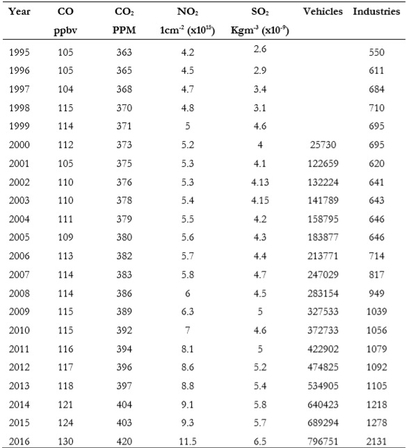

We generated a linear regression to determine the strength of relationship of industrial emissions with atmospheric pollutants and mapped the results in Figure 3.

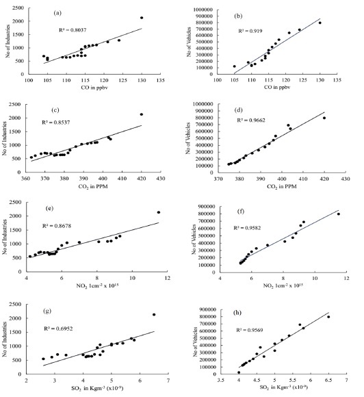
Figure 3. Linear regression model applied to various gasses (CO2, CO, NO2 and SO2) effecting the urban temperatures.
Carbon monoxide (CO) is a colorless, odorless and poisonous pollutant which is formed by fossil fuel combustions emitted by the both vehicles and the industrial emissions. The number of registered industries in Gujranwala was increased up to 2131 in the year 2016 which was only 550 in 1995. CO concentration in the atmosphere was largely influenced by industrial emissions as there were 740 industries in 1998 and the CO concentration was 115ppbv as recorded by GEOVAANI that reduced to 110ppbv against 641 industries in 2002. We applied a linear regression model to the increasing concentration of CO in comparison with temporal variation in a number of industries and the vehicles to determine the strength of relationships. We found that CO concentration in the atmosphere was largely influenced by the number of vehicles with R2=0.919 as compared to industries as mentioned in Figure 3 (a,b). CO blocks the heat and creates a natural heat island.
Carbon Dioxide (CO2) is emitted by tailpipe from trucks, cars, vehicles, and buses. As the number of vehicles increases the concentrations of CO2 increases in the atmosphere which causes the main source of heat trap in the atmosphere. The burning of fuels by vehicles add a high concentration of CO2 in the atmosphere as determined by the regression analysis applied in Figure 3 (d) with R2 = 0.96. However, industries added healthy quantity of CO2 in the atmosphere analyzed using regression analysis of CO2 with a number of industries that generated R2=0.85 in Figure 3 (c). This large concentration of CO2 in the atmosphere is capable to block terrestrial heat and to create a heat island.
Nitrogen Dioxide (NO2) is a pollutant which plays a vital role in in making ground-level ozone and particulate matter. It causes the human lungs infection and destroys the immunity system which works in defensive mode against respiratory infections such as influenza and Pneumonia. Sulphur Dioxide (SO2) is a very harmful pollutant for the human body that is produced by the burning of diesel and coal. The existence of SO2 in atmosphere is the clear indication of working of industrial plants. It is highly risky to intake by young ones that cause asthmatic attacks. We generated a correlation between temporal variations of SO2 concentration in the atmosphere in comparison to the increasing number of vehicles and industries and found a strong relationship for the both as mentioned in Figure 3 (g,h).
3. Conclusion.
Anthropogenic activities played a vital role in enhancing the concentration of atmospheric pollutants in the atmosphere of study site which has created an alarming situation not only for human survival but also for agricultural productivity. The atmosphere of Gujranwala is getting heated and this overheating has influenced the crop phenology and a seasonal shift in local climatic events, therefore, we get rainfall in Gujranwala at the time which is not suitable for crops e.g., in ripening periods. On the other hand, a large number of patients were observed in recent decade in outdoors and emergencies of hospitals who are hit sun stock, dehydration and skin problems. People face a number of health issues which are due to inhale of these pollutants. CO is a precursor of bad ozone and ozone cause skin cancer. Therefore, it is important to take bold steps at the governmental level to control the oxides of Carbon, Sulphur and Nitrogen emissions by controlling of fossil fuels and coal burning
Acknowledgement. We acknowledge earth explorer for provision of valuable data to accomplish this task.
Author’s Contribution. All the authors contributed equally.
Conflict of interest. We declare no conflict of interest for publishing this manuscript in IJIST.
Project details. NIL
References
[1] J. Voogt and T. Oke, "Thermal remote sensing of urban climates.," Remote Sens. Environ., vol. 86, p. 370–384., 2003.
[2] S. Valsson and A. Bharat, "Urban heat island: Cause for microclimate variations.," Architecture-Time Space & People,, pp. 21-25, 2009.
[3] R. Singh and A. Grover, "Remote sensing of urban microclimate with special reference to urban heat island using Landsat thermal data.," Geogr. Polonica,, vol. 87, pp. 555-568, 2014.
[4] Q. Weng, L. Dengshang and S. Jacquelyn, "Estimation of land surface temperature—Vegetation abundance relationship for urban heat island studies.," Remote Sens. Environ., Vols. 89,, p. 467–483., 2004.
[5] R. Amiri, Q. Weng, A. Alimohammadi and S. Alavipanah, "Spatial-temporal dynamics of land surface temperature in relation to fractional vegetation cover and land use/cover in the Tabriz urban area, Iran.," Remote Sens. Environ, vol. 113, p. 2606–2617, 2009.
[6] Q. H.-S. C. J. C. Le-Xiang, "Impacts of land use and cover change on land surface temperature in the Zhujiang Delta," Pedosphere,, vol. 16, p. 681–689.
[7] W. C. W. L. D. D. Y. A. Kuang, " comparative analysis of megacity expansions in China and the U.S.: Patterns, rates and driving forces," Landsc. Urban Plan, vol. 132, p. 121–135, 2014.
[8] H. S. W. Ding, "Land-use/land-cover change and its influence on surface temperature: A case study in Beijing city.," Int. J. Remote Sens, vol. 34, p. 5503–5517, 2013.
[9] S. W. N. H. E. A. R. H. Y. Jusuf, "The influence of land use on the urban heat island in Singapore.," Habitat Int, vol. 31, p. 232–242, 2007.
[10] H. Q. Z.-F. Y. X.-Y. C. Y.-B. M. W.-C. Zhang, " Analysis of land use/land cover change, population shift, and their effects on spatiotemporal patterns of urban heat islands in metropolitan Shanghai, China.," Appl. Geogr.,, vol. 44, p. 121–133., 2013.
[11] J. S. C. C. L. Z. F. M. X. W. J. Li, " Impacts of landscape structure on surface urban heat islands: A case study of Shanghai, China.," Remote Sens. Environ., vol. 115, p. 3249–3263, 2011.
[12] W. D. Y. Z. C. C. W. L. A. L. Y. Kuang, R. Zhang and J. Liu, "Quantifying the heat flux regulation of metropolitan land use/land cover components by coupling remote sensing modeling with in situ measurement.," J. Geophys. Res. Atmos., vol. 120, pp. 113-130, 2015.
[13] J. W. Y. Zhang, "Study of the relationships between the spatial extent of surface urban heat islands and urban characteristic factors based on Landsat ETM+ Data.," Sensors,, vol. 8, p. 7453–7468, 2008.
[14] R. G. A. Z. J. Singh, "Inter-seasonal variations of surface temperature in the urbanized environment of Delhi using Landsat thermal data.," Energies,, vol. 7, pp. 1811-1828, 2014.
[15] C. Q. D. Lo, "Land-use and land-cover change, urban heat island phenomenon, and health implications: A remote sensing approach.," Photogramm. Eng. Remote Sens, vol. 69, p. 1053–1063. , 2003.
[16] Y. S. J. M. C. R. A. J.-M. J. S. G. H. V. A. M. F. B. C. J. Julien, "Temporal analysis of normalized difference vegetation index (NDVI) and land surface temperature (LST) parameters to detect changes Iberian land cover between 1981 and 2001.," Int. J. Remote Sens, vol. 32, pp. 2057-2068, 2011.
[17] S. Kawashima, "Relation between vegetation, surface temperature and surface composition in the Tokyo region during winter.," Remote Sens. Environ, vol. 50, pp. 52-60, 1994.
[18] X. Z. H. L. P. Y. Z. Chen, "Remote sensing image-based analysis of the relationship between urban heat island and land use/cover changes.," Remote Sens. Environ., vol. 104, p. 133–146., (2006) .
[19] X. W. P. C. B. Zhang, "Relationship between vegetation greenness and urban heat island effect in Beijing City of China.," Procedia Environ. Sci. , vol. 2, p. 1438–1450., 2010.
[20]Y. Y. C. Q. D. J. P. Zhang, "Study on urban heat island effect based on Normalized Difference Vegetated Index: A case study of Wuhan City.," Procedia Environ.Sci., vol. 8, p. 574–581, 2012.
International Journal of Innovations in Science & Technology
February 2019 | Vol 1|Issue 1 Page | 14
[21]J. K. Y. B. B. Mallick, "Estimation of land surface temperature over Delhi using Landsat-7 ETM.," J. Indian Geophys. Union,, vol. 12, pp. 131-140, 2008.
[22]R. J. P. Sharma, "Monitoring urban landscape dynamics over Delhi (India) using remote sensing (1998–2011) inputs.," J. Indian Soc. Remote Sens., vol. 41, p. 641–650., 2013.
[23]Y. B. B. M. J. A. C. K. N. Kant, "Satellite-based analysis of the role of land use/land cover and vegetation density on surface temperature regime of Delhi, India.," J. Indian Soc. Remote Sens, vol. 37, p. 201–214., 2009.
[24]A. N. P. Acharya, "Population growth and changing land-use pattern in Mumbai metropolitan region of India.," Caminhos de Geografia, vol. 11, p. 168–185, 2004.
[25]S. Raza and S. Mahmood, "Estimation of net rice production through improvedCASA Model by addition of soil suitability constant.," Sustainability, vol. 10, no. 6, pp. 1-21, 2018.
[26]Y. Z. H. K. W. Li, "Monitoring patterns of urban heat islands of the fast-growing Shanghai metropolis, China: Using time-series of Landsat TM/ETM+ data.," Int. J. Appl. Earth Obs. Geoinf., vol. 19, p. 127–138., 2012.
[27] B. Neela, H. K. Karanam and Victor, "“Study of normalized difference built-up (NDBI) index in automatically mapping urban areas from Landsat TM imagery”," International J. Remote Sensing, vol. 8, no. 6, pp. 239-248, 2017.