
Assessment of Water Stress in Rice Fields Incorporating Environmental Parameters
Muhammad Kamran1, Sajid Rasheed Ahmad1, Khurram Chohan2, Azeem Akhtar3*, Amna Hassan4, Rao Mansoor Ali Khan5
1 University of the Punjab PU · College of Earth and Environment sciences.
2 Government College University, Lahore.
3 Department of Space Science University of the Punjab Lahore
4 The Islamia University of Bahawalpur.
5 University of Minnesota USA.
* Correspondence: Muhammda Kamran, iamkamee@gmail.com
Citation | Kamran.M, Ahmad.R.S, Chohan.K, Akhtar.A, Hassan.A, Khan.A.M.R, “Assessment of Water Stress in Rice Fields Incorporating Environmental Parameters.”. International Journal of Innovations in Science and Technology. Vol 4, Issue 2, 2022, pp: 416-424
Received |April 13, 2022; Revised | April 25, 2022; Accepted | April 28, 2022; Published | April 30, 2022.
________________________________________________________________________
Rice is considered as a major crop due to its demand globally. Pakistan is famous throughout the world to produce export quality rice which have healthy contribution in boosting the regional economy. Rice plant require plenty of water for its proper growth and development therefore, water conservation is significant to maintain water reserves for a sustainable future. The main objective of this study was to identify day-to-day availability of water in rice fields from Germination to Ripening (GTR) using Carnegie Ames Stanford Approach (CASA) model. CASA model incorporates real-time parameter e.g., temperature, pressure, extraterrestrial radiations, Leaf Area Index (LAI), vapor pressure and sunshine hours to compute net-shortwave radiations (Rns), net-longwave radiations (Rnl), net-radiations (Rn), actual incoming radiations (Rso), sensible heat flux (H), ground heat flux (Go) and finally the water stress (W). The averaged values of Rn, Rso, Rns, Rnl and H were computed as 206, 319, 178, 34 and 124 (wm-2) respectively for GTR. Total expected sunshine hours were 1584h but we could receive only 874 h during GTR due to “off and on” cloud activity. LAI and Go were observed in inverse relation to each other. Rn, H and Go were used to compute the availability of water during GTR and concluded that the experimental site had surplus of water in early growth stages of rice crop having “W>0.5”, while milky dough and ripening stages were observed under water deficit (W<0.5). The results computed through CASA model were in accordance with actual observations collected through field survey up to 86%.
Keywords. Shortwave radiations; CASA Model; Net radiations; Sensible Heat Flux, Ground heat flux.
INTRODUCTION
Rice (Oriza stavia L) is accounted as widely grown crop after wheat, over vast lands throughout the world [1]. Irrigated rice is an essential part of food security[2]. Rice is known as water baby, which needs excess amount of fresh water throughout its life cycle for its proper growth and development [3]. Various human activities are responsible for fresh water turbidity for instance industrial discharge, solid waste and the domestic discharge [3]–[6]. Asian countries are contributing about 90% in global rice production with utilization of 91% of global fresh water. It is projected that 15 M Ha of irrigated land and 22 M Ha of dry rice area may face water scarcity by 2025 [7]. Fresh water is essential to achieve targeted yield therefore, water saving techniques are of great importance for a sustainable and green future. Many researchers have devised a number of techniques to manage water supply in optimized range to receive healthy yield [8], [9]. All these techniques are related to the sustainable use of water. The main objectives of researches, which were performed in context of crop-water relationship, were to increase net crop production with less amount of water.
Numerous factors are responsible to enhance productivity by provision of water in reasonable quantity e.g., soil type, soil pH and electric conductivity of soil [10]. Sand is not considered suitable for rice crop because it is perfectly drained. However, sandy clay is well drained therefore, considered less suitable while clay is best for rice cultivation because it is imperfectly drained and hold water for long times [11]. The clayish land has highest water holding capacity, so we can save a large amount of water with changing soil type [12]. The suitable range of electric conductivity for rice fields is 0.75-1.50 and the pH of soil must be between 5.4 and 7.1 pH [10].
Computation of water stress is a component of CASA model that initially requires various solar fluxes affecting crop growth and development which are based on sunlight and termed as Light Use Efficiency (LUE). The LUE directly affect water intake capacity of the crops. CASA model has been proved efficient to map productivity at global scales by fixing solar radiations [13]. Every crop needs certain amount of light for proper growth and development [11]. LUE is a very basic property of a plant [14] which express heterogeneity. The light used by plants is dependent upon a number of factors e.g. availability of chlorophyll content, leaf age, light intensity and crop’s developmental stage. Solar zenith angle, shape of crop canopy, leaf inclination angle and the leaf area are considered most influencing factors while computing the light used by plants. Dissimilar species are distinguished by computation of their light used throughout their life cycle [15], [16]. There are many methods commonly used to compute light use efficiency including Eddy Covariance method [17], Quantum efficiency Renocking method and the productivity inversion method [18]. Photo Reflection Index (PRI) [19] is widely used to compute the variations in the light used by various crops while site-based measurements had been taken commonly to compute the LUE in the previous decades.
This research aims at investigating rice fields suffering from water stress by incorporating various environmental factor essential for growth and development of rice crop e.g., temperature, pressure, sunshine hours and actual vapor pressure. It also aims at computation of variations in various fluxes throughout the rice growth period which effects the crop growth and development. These fluxes include net shortwave radiations (Rns), net longwave radiations (Rnl), net radiations (Rn), possible incoming radiations (Rso), sensible heat flux (H), ground heat flux (Go) and actual incoming radiations (Ra). CASA model incorporates Rns, Rnl, Rn, Rso, H, Go and Ra to provide water availability in rice fields on daily basis.
Study site
Hafizabad district was selected to execute this research. This district produces the rice of export quality. The study site is located at latitude between (31.4-32.2)oN and longitude between (73-73.5)oE. Monsoon directly hit the study site therefore, it receives large amount of water as rainfall which is good for rice cultivation. Water is distributed through connected network of water channels in an organized way. Weather is very severe where temperature vary from 0oC in winter to 48oC in summer. The study site is mapped in Figure 1.
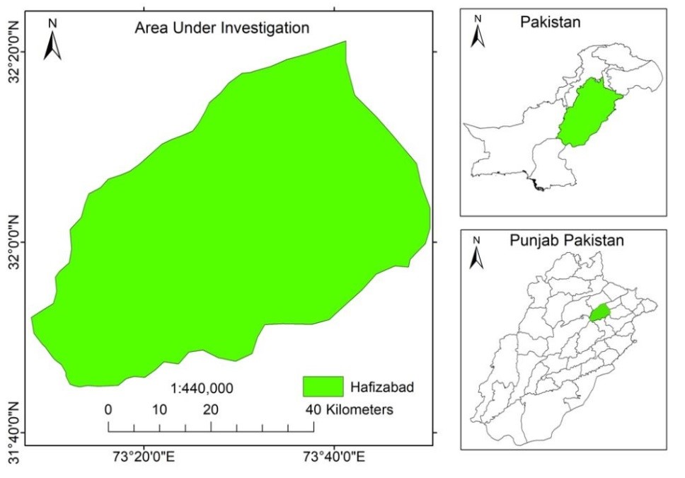
Figure 1. Study site.
The methodology to accomplish this research is described in Figure 2.
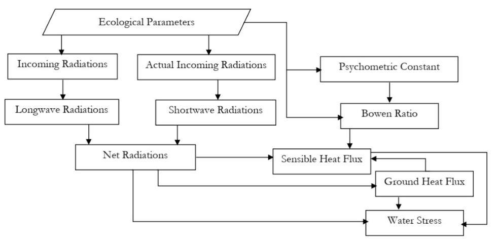
Figure 2. Flow of methodology.
The basic environmental factors which were used to compute water stress in rice fields included daily fluctuation in temperature, possible sunshine hours, pressure, extra-terrestrial radiations, LAI, actual sunshine hours and the albedo of rice crop.
The growth and development of crops is derived by sunlight [20] which is computed by estimation of Net radiations (Rn). Rn shows the integrated impact of incoming shortwave radiations (Rns) and the earth’s emitted longwave radiations (Rnl). Net Radiations effects the process of evapotranspiration therefore; it is important to compute Rn to review agro-climatic interactions [21]. Mathematically, Rn cab be computed as below [22],
![]() (1)
(1)
Where Rns are net shortwave or incoming radiations, while Rnl are net longwave or outgoing radiations. Shortwave radiations are normally computed by incorporating albedo and actual incoming radiations [22].
![]() (2)
(2)
Where α is the albedo of rice crop which is normally taken between a range of 0.15 -
0.25 [23]–[25]and Rs represents the possible incoming solar radiations.
Rnl can be computed using the expressions as follows [27],
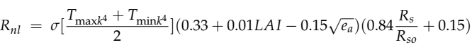 (3)
(3)
Where is Stephan Boltzmann’s constant and it’s value is 4.09 -9MJ/k4M2. Tmax and Tmin are daily fluctuations in temperature from GTR, Rso is the actual solar flux while ea is the actual vapor pressure. We obtained Tmin, Tmax, and ea from local metrological station. Extra-terrestrial radiations are represented by Ra. Ra is the solar flux which is recorded at the outermost boundary of our atmosphere [26]. Ra depends upon solar angle that changes from January to December. Ra from GTR, was estimated using the website as below, http://www.engr.scu.edu/~emaurer/tools/calc_solar_cgi.pl.
The actual solar flux that approached the earth’s surface by its interaction with clouds and other atmospheric contents are known as actual incoming solar radiations which were computed using the expression as below [22].
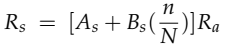 (4)
(4)
In equation 4, there are two calibration constants, As and Bs and the value of these constants is fixed as 0.25 and 0.50 respectively, N and n represents the possible sunshine hours and actual sunshine hours respectively. We acquired n, N from local metrological stations.
If there is sunny day, even then about 25% radiations are scattered by their interactions with atmospheric gases and 75% approaches the surface of the earth. Rso can be computed according to Angstrom’s expression as below [28]
![]() (5)
(5)
Ground heat flux (Go)
Ground heat flux (Go) describes the penetration of heat in to the soil. It defines the heat conduction capacity of soil through which it is travelling that depends upon the concentration of various heat conducting elements present in a particular soil. Go actually control all bio-chemical reactions occurring in soil. The value of Go is very small therefore, it is ignored but it may create considerable errors sometime. Go was estimated using the expression as below [29],
![]() (6)
(6)
Where LAI is the leaf area index and Rn is the net radiations. Go is largely affected by LAI because an increase in LAI reduces the heat to reach the surface of earth and minimum leaf area at the time of germination leads to direct approach of sunlight in to the soil where it is grown. Go is minimum where the crop has maximum leaf area. In the study site, Go was observed minimum in the month of September where the leaf area reached at 6.65 m2 m-2. We obtained 20 field observations to record leaf area of the rice crop from July to October with a 5-days temporal window as shown in Figure 3.
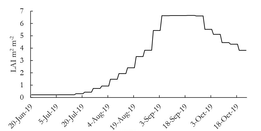
Figure 3. Temporal changes in LAI throughout the rice growth period.
We fixed a 5 Days window between successive readings of leaf area because a leaf takes about 5 days to grow in considerable limits. Same temporal window was fixed by [11] to estimate the net rice production using CASA model.
Sensible heat flux (H)
Sensible heat is defined as the transfer of heat energy required for a plant to balance its temperature in accordance to its environment. It is difficult to compute the sensible heat flux accurately [30] therefore, it is taken as residual of energy balance [31].Bowen ratio (β) plays a vital role for computing H. Bowen ratio can be computed by taking a ratio of variations in vapor pressure and temperature of rice crop canopy using the expression as below,
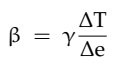 (7)
(7)
Where γ is a psychometric constant and its value can be computed using the expression as below [32]
![]() (8)
(8)
Variations in actual vapor pressure, temperature and pressure were acquired from local weather station and the sensible heat was computed using Bowen Ratio [31] as below,
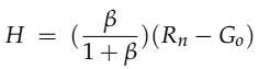 (9)
(9)
Where β, Rn and Go are Bowen ratio, net radiations and the ground heat flux respectively.
Water stress (W) determine the amount of available moisture content in soil. Water stress can be computed by the following expressions as below [33].
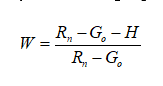 (10)
(10)
W vary between 0 and 1, where W=0 represents the oven dry soil and w = 1 shows the surplus of water [34] – [38].
Results and Discussion
Rn, Rns, Rnl, and Rso were computed and the results are mapped in figure 4
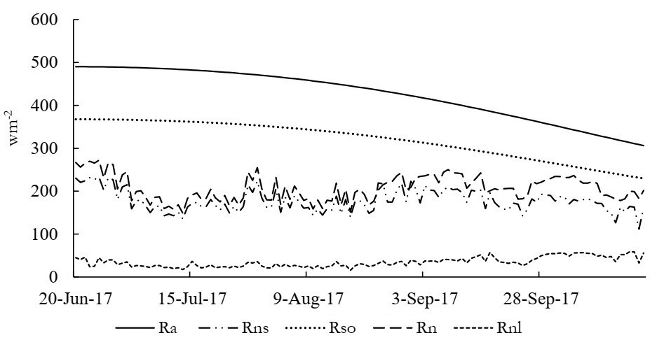
Figure 4. Fluctuations in various solar fluxes throughout the rice crop life cycle.
Figure 4 is showing fluctuations in different fluxes faced by rice canopy throughout the rice crop lifecycle. Rice germination started on June 20, 2019 and harvesting of the rice crop ended on October 20, 2019. During this period, the extraterrestrial radiations were declined due to change in solar angle. About 55640 wm-2 were received on the outer boundary of our atmosphere during 120 days of rice crop growth but we could actually receive a flux of 27470 wm-2 that approached the rice crop canopy. The averaged estimates of Ra, Rso, Rns, Rnl and Rn were computed as 426 wm-2, 319 wm-2, 178 wm-2, 34 wm-2 and 206 wm-2 throughout the rice crop life cycle. Figure 4 is showing many peaks and dips in Rn, Rns, and Rnl that resemble with the shape of n/N mapped in Figure 5. The fluctuations in Figure 5 show that as the value of n/N approaches to 1, it represents a sunny day and its value near to zero represents a cloudy day.
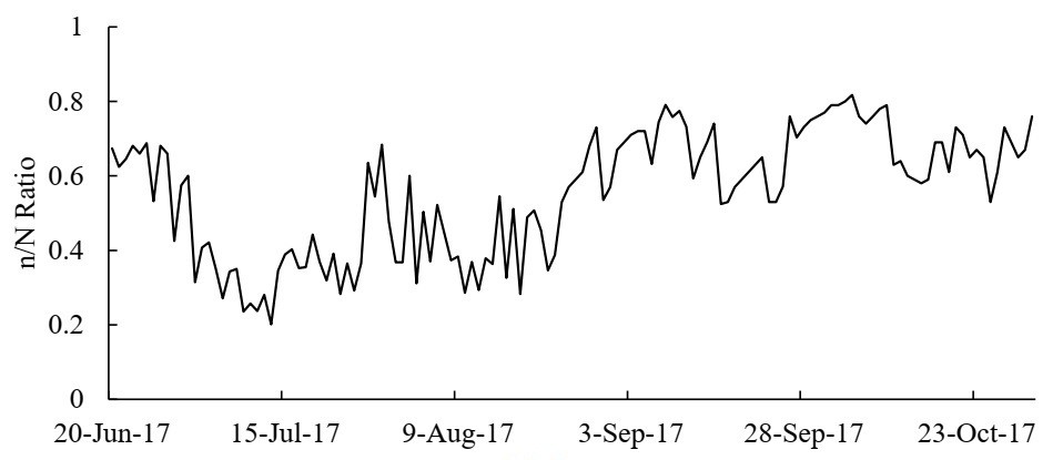
Figure 5. Variations in actual and possible sunshine hours.
Figure 5 is showing that cloud activity throughout the life cycle of rice crop. We observed that the value of n/N must be near to zero in early growth stages of rice crop which express sever cloud activity and probably the rainfall, while it must be near to 1 in milky dough and ripening stages that results in sunshine situation which is good for ripening of rice crop properly. Figure 5 is showing that a total possible sunshine hour, which were expected to approach the rice crop canopy were 1584 h but we could receive only 874 h throughout the rice crop cycle due to cloudy situation on the study site.
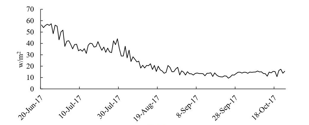
Figure 6. Ground heat flux throughout the rice crop life cycle.
Figure 6 was mapped by putting Rn and LAI using equation 6 which is showing a decreasing trend. The gradual decline to Go curve is due to increase in LAI. As leaf area increases, it stops heat to penetrate and to approaches the ground. We computed fluctuations in ground heat flux and the results are shown in Figure 6.
We applied a regression of second order to LAI and Go and found R2=0.8843 as shown in Figure 7.
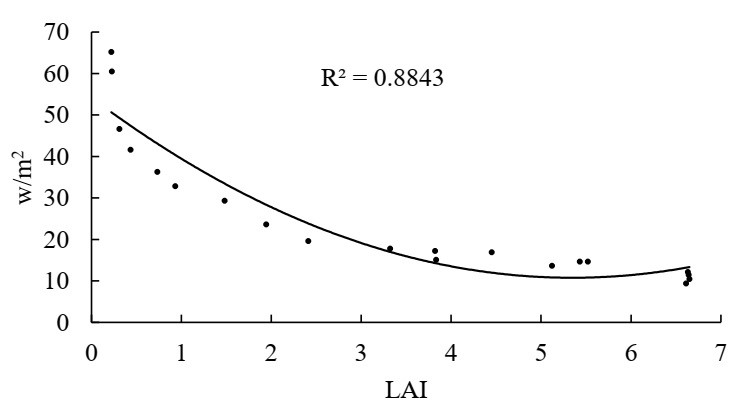
Figure 7. A 2nd order correlation between LAI and Go.
We computed the sensible heat flux of rice crop by putting the values of Bowen ratio (β), Rn and Go in Equation (9) and the results are shown in Figure 8 as below
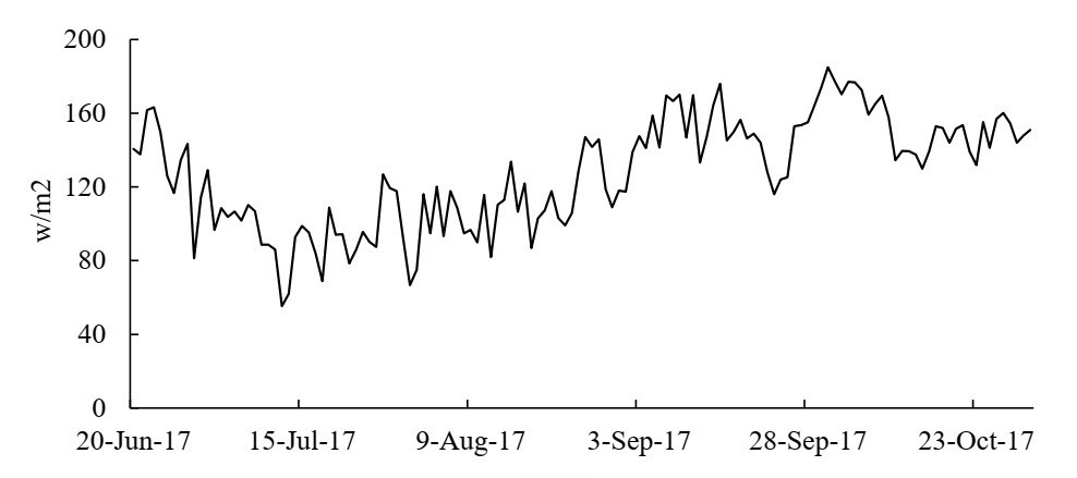
Figure 8. Fluctuations in H throughout the rice crop life cycle.
The shape of curve in Figure 8 resembles with the shape of Rn curve in Figure 4. It is due to the reason that H and Rn are in direct relationship, as Rn increases, it need more heat for a plant to maintain its body temperature therefore, H increases. Sensible heat flux throughout the RLC was recorded as 124 wm-2 as averaged. We computed water stress in rice fields on daily basis using Go, H and Rn in Equation 10 and the results are shown in Figure 9
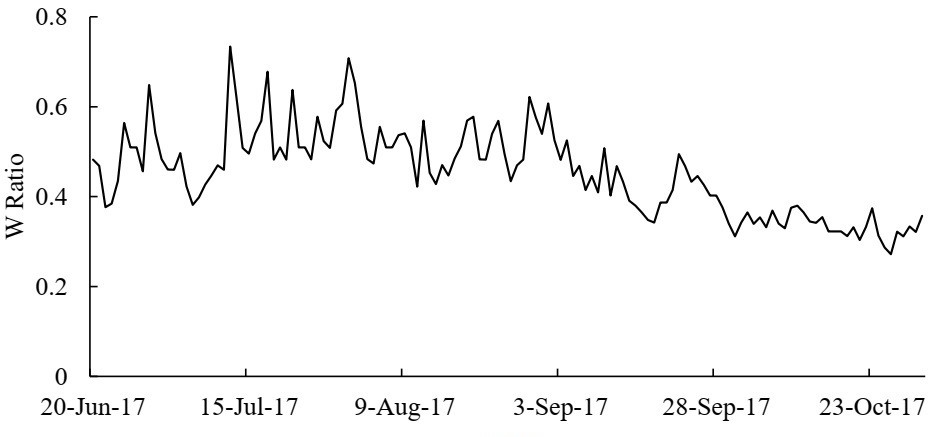
Figure 9. Water stress throughout the rice crop life cycle.
Figure 9 shows that day where curve descends to zero below 0.5, it represents deficiency of water in rice fields, in comparison to the day where the curve crosses 0.5 toward 1. The study site had excess of water (W>0.5) in germination, leaf emergence, tillering and panicle primordia initiations while the literal stages of growth were in water stress (W<0.5). On visiting the fields, we found that ripening stage of rice crop is water free stage while initial stages need penalty of water for proper development. Finally, we observed that all crop growth factors Rn, Rns, Rnl, Go, H and W are largely affected by the cloud activity (n/N). The curve in figure 9 is representing, if w<0.5, there is water stress and vice versa.
Conclusion:
Both monitoring and evaluations of environmental parameters (i.e. temperature, pressure, actual vapor presser and extraterrestrial radiations) play a vital role to understand the sequential growth stages of rice crop for optimum water use. One can determine the deficiency or penalty of water in rice fields by incorporating real-time ecological parameters. CASA based methodology was adopted to accomplish this research which is handy to apply at global scales to monitor the rice crop in a better way.
References:
[1] M. Saifullah et al., “Estimation of Water Stress on Rice Crop Using Ecological Parameters.,” Int. J. Agric. Sustain. Dev., vol. 01, no. 01, pp. 17–29, 2019, doi: 10.33411/ijasd/20190103.
[2] J. Yang and J. Zhang, “Crop management techniques to enhance harvest index in rice,” J. Exp. Bot., vol. 61, no. 12, pp. 3177–3189, 2010, doi: 10.1093/jxb/erq112.
[3] A. K. Thakur, S. Rath, D. U. Patil, and A. Kumar, “Effects on rice plant morphology and physiology of water and associated management practices of the system of rice intensification and their implications for crop performance,” Paddy Water Environ., vol. 9, no. 1, pp. 13–24, 2011, doi: 10.1007/s10333-010-0236-0.
[4] B. A. M. Bouman, “A conceptual framework for the improvement of crop water productivity at different spatial scales,” Agric. Syst., vol. 93, no. 1–3, pp. 43–60, 2007, doi: 10.1016/j.agsy.2006.04.004.
[5] T. Chapagain, A. Riseman, and E. Yamaji, “Assessment of System of Rice Intensification (SRI) and Conventional Practices under Organic and Inorganic Management in Japan,” Rice Sci., vol. 18, no. 4, pp. 311–320, 2011, doi: 10.1016/S1672-6308(12)60010-9.
[6] S. D. Khepar, A. K. Yadav, S. K. Sondhi, and M. Siag, “Water balance model for paddy fields under intermittent irrigation practices,” Irrig. Sci., vol. 19, no. 4, pp. 199–208, 2000, doi: 10.1007/PL00006713.
[7] H. J. Nesbitt, “Rice Production in,” World, vol. 12, no. 2, pp. 186–191, 1997.
[8] V. J. Pascual and Y. M. Wang, “Utilizing rainfall and alternate wetting and drying irrigation for high water productivity in irrigated lowland paddy rice in Southern Taiwan,” Plant Prod. Sci., vol. 20, no. 1, pp. 24–35, 2017, doi: 10.1080/1343943X.2016.1242373.
[9] A. S. Kima, W. G. Chung, Y. M. Wang, and S. Traoré, “Evaluating water depths for high water productivity in irrigated lowland rice field by employing alternate wetting and drying technique under tropical climate conditions, Southern Taiwan,” Paddy Water Environ., vol. 13, no. 4, pp. 379–389, Oct. 2015, doi: 10.1007/S10333-014-0458-7.
[10] S. M. H. Raza, S. A. Mahmood, A. A. Khan, and V. Liesenberg, “Delineation of Potential Sites for Rice Cultivation Through Multi-Criteria Evaluation (MCE) Using Remote Sensing and GIS,” Int. J. Plant Prod., vol. 12, no. 1, pp. 1–11, 2018, doi: 10.1007/s42106-017-0001-z.
[11] S. M. H. Raza and S. A. Mahmood, “Estimation of net rice production through improved CASA model by addition of soil suitability constant (hα),” Sustain., vol. 10, no. 6, 2018, doi: 10.3390/su10061788.
[12] M. M. Waqar, F. Rehman, and M. Ikram, “Land suitability assessment for rice crop using geospatial techniques,” Int. Geosci. Remote Sens. Symp., no. July 2013, pp. 2844–2847, 2013, doi: 10.1109/IGARSS.2013.6723417.
[13] H. Wang, X. Li, H. Long, and W. Zhu, “A study of the seasonal dynamics of grassland growth rates in Inner Mongolia based on AVHRR data and a light-use efficiency model,” Int. J. Remote Sens., vol. 30, no. 14, pp. 3799–3815, 2009, doi: 10.1080/01431160802552702.
[14] J. B. Bradford, J. A. Hicke, and W. K. Lauenroth, “The relative importance of light-use efficiency modifications from environmental conditions and cultivation for estimation of large-scale net primary productivity,” Remote Sens. Environ., vol. 96, no. 2, pp. 246–255, May 2005, doi: 10.1016/J.RSE.2005.02.013.
[15] D. E. Ahl, S. T. Gower, D. S. Mackay, S. N. Burrows, J. M. Norman, and G. R. Diak, “Heterogeneity of light use efficiency in a northern Wisconsin forest: Implications for modeling net primary production with remote sensing,” Remote Sens. Environ., vol. 93, no. 1–2, pp. 168–178, Oct. 2004, doi: 10.1016/J.RSE.2004.07.003.
[16] W. Zhu, Y. Pan, H. He, D. Yu, and H. Hu, “Simulation of maximum light use efficiency for some typical vegetation types in China,” Chinese Sci. Bull., vol. 51, no. 4, pp. 457–463, 2006, doi: 10.1007/s11434-006-0457-1.
[17] X. Xiao et al., “Satellite-based modeling of gross primary production in a seasonally moist tropical evergreen forest,” Remote Sens. Environ., vol. 94, no. 1, pp. 105–122, Jan. 2005, doi: 10.1016/J.RSE.2004.08.015.
[18] Pei, B.; Yuan, Y.; Jia, Y.; Wang, W.; Josef, E 2000. A study on light utilization of poplar crop intercropping system. Sci. Silvae Sin., 36, 13–18, doi: 10.11707/J.1001-7488.20000303.
[19] F. G. Hall et al., “Multi-angle remote sensing of forest light use efficiency by observing PRI variation with canopy shadow fraction,” Remote Sens. Environ., vol. 112, no. 7, pp. 3201–3211, Jul. 2008, doi: 10.1016/J.RSE.2008.03.015.
[20] J. L. Monteith, “Solar Radiation and Productivity in Tropical Ecosystems,” J. Appl. Ecol., vol. 9, no. 3, p. 747, Dec. 1972, doi: 10.2307/2401901.
[21] Zhu, W.; Pan, Y.; He, J.; Yu, D.; Hu, H. 2006 Simulation of maximum light use efficiency for some typical vegetation types in China. Chin. Sci. Bull., 51, 457–463. .
[22] B. Wu, S. Liu, W. Zhu, N. Yan, Q. Xing, and S. Tan, “An Improved Approach for Estimating Daily Net Radiation over the Heihe River Basin,” Sensors (Basel)., vol. 17, no. 1, Jan. 2017, doi: 10.3390/S17010086.
[23] P. G. Oguntunde, O. J. Olukunle, O. A. Ijatuyi, and A. A. Olufayo, “A semi-empirical model for estimating surface albedo of wetland rice field,” Agric. Eng. Int. CIGR J., no. May 2014, 2007.
[24] J. L. Tsai, B. J. Tsuang, P. S. Lu, M. H. Yao, and Y. Shen, “Surface energy components and land characteristics of a rice paddy,” J. Appl. Meteorol. Climatol., vol. 46, no. 11, pp. 1879–1900, 2007, doi: 10.1175/2007JAMC1568.1.
[25] T. W. Giambelluca, D. Hölscher, T. X. Bastos, R. R. Frazão, M. A. Nullet, and A. D. Ziegler, “Observations of albedo and radiation balance over postforest land surfaces in the eastern Amazon Basin,” J. Clim., vol. 10, no. 5, pp. 919–928, 1997, doi: 10.1175/1520-0442(1997)010<0919:OOAARB>2.0.CO;2.
[26] M. Irfan, Z.-Y. Zhao, M. Ahmad, and M. Mukeshimana, “Solar Energy Development in Pakistan: Barriers and Policy Recommendations,” Sustainability, vol. 11, no. 4, p. 1206, 2019, doi: 10.3390/su11041206.
[27] W. Munley and L. Hipps, 1991 Estimation of regional evaporation for a tallgrass prairie from measurements of properties of the atmospheric layer., Water Resour. Res., vol. 27, p. 225–230.,.
[28] Angstrom, 1924 Solar and terrestrial radiation., Q. J. R. Meteorol. Soc. , vol. 50, pp. 121-125,.
[29] Tasumi, M. 2003; Progress in Operational Estimation of Regional Evapotranspiration Using Satellite Imagery. Ph.D. Thesis, University of Idaho, Moscow, ID, USA, p. 357.
[30] Sauer, T.J.; Horton, R. Soil Heat Flux; 2005, University of Nebraska Lincolon: Lincoln, NE, USA, Volume 47, pp. 131–154. Available online: http://digitalcommons.unl.edu/usdaarsfacpub
[31] Bowen, I.S. 1926 The ratio of heat losses by conduction and by evaporation from any water surface. Phys. Rev.J. Achive, 27, 779–787
[32] Zotarelli, L.; Dukes, M.D.; Romero, C.C.; Migliaccio, K.W.; Morgan, K.T. 2015, Step by Step Calculation of the Penman-Monteith Evapotranspiration (FAO-56 Method); IFAS University of Florida: Gainesville, FL, USA
[33] Tanner, C.B 1960, Energy balance approach to evapotranspiration from crops. Soil Sci. Soc. Am. Proc. 24, 1–9
[34] Sajid. M, Mohsin. M, Jamal. T, Mobeen. M, Rehman. A, Rafique A, “Impact of Land-use Change on Agricultural Production & Accuracy Assessment through Confusion Matrix”. International Journal of Innovations in Science & Technology, Vol 04, Issue 01: pp; 233- 245, 2022.
[35] Akram. F, Fatimah. T, Jamal. T, Saleem. M. U, Javed. H, Sharif. S, Yousaf. K, Khan. N. I, Karamat. A, “Salinity and Fertility Status of Irrigated soils in District Nankana Sahib, Punjab, Pakistan”. International Journal of Innovations in Science & Technology. Vol 4, Issue 1, pp: 213-221, 2022.
[36] Farhan. S. M, Arif. H, Ahmad. H. H, “Estimation of relation between moisture content of soil and reflectivity index using GPS signals”. International Journal of Innovations in Science & Technology, Vol 03 Issue 04: pp 218-227, 2021.
[37] Younis. H, Arshed. M. A, Hassan. F, Khurshid. M, Ghassan. H, “Tomato Disease Classification using Fine-Tuned Convolutional Neural Network”. International Journal of Innovations in Science & Technology. Vol 4, issue 1, pp: 123-134, 2022.
[38] Khan. R. M. A, Naqvi. S. B, Rana. Q. S, Mahmood. S. A, Rasheed. M, “Detecting Aphid Concentration in Wheat Leaf Using Remote Sensing and GIS”. International Journal of Innovations in Science & Technology, Vol 4, Issue 2, 2022, pp: 336-347
 |
Copyright © by authors and 50Sea. This work is licensed under Creative Commons Attribution 4.0 International License. |