
Blind Image Deblurring Using Laplacian of Gaussian (LoG) Based Image Prior
Sofia Zaka1, Muhammad Nadeem Majeed2, Hassan Dawood3
1,2,3 University of Engineering and Technology Taxila, Punjab Pakistan.
* Correspondence: Sofia Zaka, Email ID: sofiazaka916@gmail.com.
Citation | Zaka. S, Majeed. M. N, Dawood. H, “Blind Image Deblurring Using Laplacian of Gaussian (LoG) Based Image Prior”, International Journal of Innovations in Science and Technology, Vol 4, Issue 2, 2022, pp 365-374.
Received | March 10, 2022; Revised | March 29, 2022; Accepted | April 21, 2022; Published | April 23, 2022.
Blind image deconvolution, a technique for obtaining restored image as well as the blur kernel from an inexact image. This research uses spatial characteristics to tackle the problem of blind image deconvolution. To work, the proposed method does not necessitate prior information about the blur kernel. Many applications, such as remote sensing, astronomy, and medical X-ray imaging, necessitate blind image deconvolution algorithms. This study used the maximum a posteriori (MAP) paradigm to create a new blind deblurring approach for removing blur from images. In beginning, we employed a Laplacian of Gaussian (LoG)-based image before regularising the gradients of an image. In the second phase, we used an operator known as the Iterative Shrinkage Thresholding Algorithm (ISTA) to cope with the non-convex challenge that develops during the entire deblurring procedure. Finally, we compared our method to several well-known methods in terms of quantitative and qualitative qualities, and we were able to determine which strategy was the most effective. Our findings show that the strategy we propose outperforms the others by a large margin.
Keywords: Blind Image Deblurring (BID), Blind Deconvolution, Maximum Posterior (MAP), Laplacian of Gaussian (LoG).
INTRODUCTION
It is possible to deconvolve a blurred image into its original form without any knowledge of the actual image or the process that leads it to be blurred, known as a point spread function (PSF). Pixel's intensity is affected by the intensity of adjacent pixels due to motion artifacts, lens flaws, and air changes such as turbulence, all of which can cause blur[1]. The recorded image is typically corrupted by arbitrary noise generated by an optical device, resulting in measurement errors[2]. There are two phases involved in producing a blurred image: convolution and deconvolution of the PSF from the blurred image[3]. Video conferencing, diagnostic imaging, and celestial imaging all require this blind deconvolution, but it is difficult or impossible to calculate the PSF before the operation, which makes Blind Image Deblurring(BID) the process of obtaining a true image from its distorted form, a challenging task.
It is possible to utilize blind (BD), non-blind (NBD), or semi-blind (SBD) deconvolutions depending upon whether or not you know the PSF shape. BD deconvolution approaches such as statistically significant blind deconvolution with a Gauss-Newton procedure [4] and peak restoration blind deconvolution [5] involve a simultaneous estimate of spectrum data and blur kernel from observed data. It makes blind deconvolution a challenging task, and noise makes it even more difficult. The Fourier self-deconvolution (FSD) approach [6], the most frequent approach used during infrared spectroscopy, and the maximum Burg entropy (MaxEntD) method [7], which presently has good performance in deconvolution of absorption spectra, can be employed for spectrum restoration when the PSF is known. In contrast, PSF is rarely encountered in real-world applications. There will be bad results if the blur kernel is incorrectly supposed to be different from the actual one. PSF is assumed to be parametric in semi-blind deconvolution approaches like semi-blind deconvolution based on several regularizations [8].
Maximum Posterior (MAP), Variational Bayesian, and edge prediction are the three types of blind deconvolution algorithms. The computational cost of VB-based methods is higher than MAP, but it can avoid trivial solutions. Salient Structures-Based Kernel Estimation and Sparse Regularization-Based Kernel Estimation are two variants of kernel estimation based on MAP that have been proposed.
From a blurred input, the purpose of blind image deblurring is to restore a blur kernel and a sharp latent image. It's a classic vision problem, and there's been a lot of progress in recent years. A convolution operation can be used to model the blurring process when it is spatially invariant:
![]() (1)
(1)
Where b represents blur image, l for latent image, k for blur kernel, n for noise, and * denotes the convolution operator between them. Restored images appear to be of low quality when image structures are too small to fit inside the blur scale. A new blind deconvolution algorithm based on Laplacian of Gaussian based regularization is proposed to overcome this problem in this paper. We have proposed an image deblurring method based on salient detection, which removes damaging picture structures from the estimation of blurry kernels. Other non-uniform deblurring and priors can be solved using the approach we've devised, as we show here. The results of this research show that the suggested method outperforms currently used blind image deconvolution methods. An image that has been enhanced by using this method has a better value on evaluation parameters such as peak signal to noise ratio (PSNR) and structural similarity index measure (SSIM), than those obtained using other methods, according to experiments on improving blurred photos.
The rest of this document is structured as follows. In Section 2, we describe our blind deconvolution model, the priors we utilized, and the reasoning behind our choice. There follows a description of how the proposed approach is optimized and the algorithm is implemented. This section also explains the proposed algorithm's convergence features. The quantitative and qualitative results are presented in Section 3 for comparison with some other common methods of image restoration. The concluding paragraphs are included in the last section.
PROPOSED METHODOLOGY
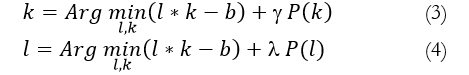
The blind image deblurring challenge can be approached iteratively by estimating alternate iterations of the transitional latent image and the blur kernel. This optimization scheme will be used to develop a new blind deblurring technique, which will be discussed in this section. Using the MAP framework, after blurring y, we extracted two factors including latent image and blur kernel. Deblurring was computed using the equation below:
![]() (2)
(2)
In (2), ‘P’ denotes prior for k and latent image, both denotes the weights.
A new way of solving the latent image is used to solve the deblurring process, which is conceptualized as an optimization problem.
In our model, we employed the Laplacian of Gaussian (LoG) which is used to calculate the image prior, during each iteration we use the previously calculated blur kernel to estimate a final blur kernel. Using the resulting blur kernel, a latent image recovery method is implemented. The complete methodology is shown in Figure 1 and the algorithm is shown in Algorithm 1.
Algorithm 1: Overall Deblurring Algorithm
Result: Latent Image and estimated kernel
Input: blurred image b, kernel size h, derivative filters, a high-frequency image I.
(Two main parts of Blind Image Deblurring algorithm)
Apply loop on coarser levels:
For i< tmax+1 do
- Estimate l by using subsection A
- Estimate k by using subsection B
End for
Using the Non-Blind Deconvolution part to obtain a final recovered image
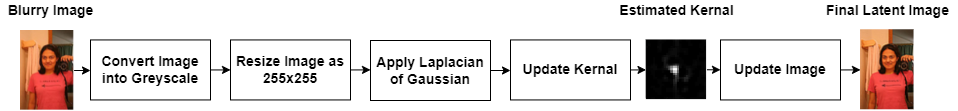
Figure 1. Methodology of Our Model.
Updating Latent Image
Using the previous iteration's blur kernel k, we will use Laplacian of Gaussian (LoG) to estimate the intermediate latent image .
![]()
The Laplacian is a two-dimensional isotropic metric of the second spatial derivative of that image. The Laplacian of an image reveals regions of fast intensity change, and as a result, it is frequently employed for edge identification in images. It is common practice to apply the Laplacian to an image that has already been smoothed with something that approximates the Gaussian smoothing filter in terms of reducing the image's susceptibility to noise. As LoG is a combination of Laplacian and Gaussian, so, here is a mathematical form of a simple Laplacian function.
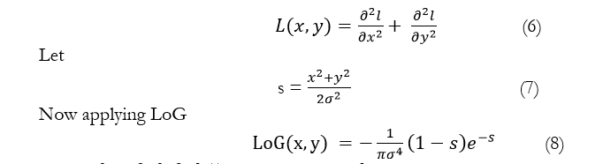
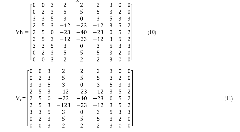
In (5), =( h , v )T is the gradient of .
In(7), (8), is the standard, deviation. In this research, we have used to obtain hand v. Now we have introduced another term for vertical and horizontal gradients, in the above equation as follows:
= h, v ]T
Now (5) will look like this,
![]()
In (9), is the penalty-related parameter, when is close to infinity, the result of (9) will be similar to the result of (5). We then work on (9) by updating and independently of one another, in this equation we keep the variable constant.
We begin by setting the value of d to zero. Each iteration of the process will result in being obtained by (12),
To address the general linear inverse issue, the Iterative Shrinkage Thresholding Algorithm (ISTA) is utilized. ISTA is a very basic and fast algorithm that only requires multiplying the matrix K with the vector image , and then it shrinks each component one by one. In our latent image update algorithm, we just use ISTA stride as the inner iteration. In this algorithm represents soft shrinkage operator.
![]() (17)
(17)
Algorithm 2: Iterative Shrinkage Thresholding Algorithm (ISTA)
Result: Image j
Input: k, , b, max, 0, t
for i=0 to j-1, do
end
Updating Kernel

To determine the kernel k, we built an image pyramid using a fine technique. The transitional latent image from the preceding finer level was used to set the variable k whenever a pyramid level is started. Each pyramid level has 10 repetitions between k and for the sake of this demonstration. Once a cycle is complete, we select an adjustment strategy to use. Algorithm 3 depicts the primary procedures required in obtaining the blur kernel k at a single pyramid level. In this research, we can extract the final latent image by using (2).The algorithm for kernel estimation is as follows
Algorithm 3: Image kernel Estimation
Result: Updated Kernel k, latent image
Input: b
Initialize k
for j=0 to 20, do
Estimate image by Algorithm 1
Estimate kernel by equation (18)
end
EXPERIMENTAL RESULTS AND DISCUSSION
In this section, we have discussed the datasets used to obtain the results and the evaluation parameter selection is discussed for the evaluation of our method. After that, the results of our method are evaluated using these evaluation parameters and then they are shown and recorded.
Dataset
To demonstrate the usefulness of the suggested method, results are collected for both real-world and synthetic images using well-known evaluation parameters to demonstrate its effectiveness. For the synthetic dataset, we use Levin et al. dataset[9] and the other dataset is the Kohler et al. [10] dataset. The details of these datasets are given in the next sections.
Evaluation Metrics
The PSNR, SSIM, and the time in seconds were used to evaluate the performance of the LoG-based approach, which are considered well-known evaluation parameters. We calculated PSNR using the following equation:

In (23) , represents means, variances, and covariance respectively. represent constants. “x” and ‘y’ show recovered image and original image respectively.
Performance evaluation on Synthetic Dataset
We chose the Levin et. al dataset. This dataset contains four images and each image contains eight different blur kernels. After convolution of kernel and images, we obtain 32 different images of different sizes. The size of the kernels varies from 3×3 to 27×27. This dataset includes ground truth images, ground truth kernels, and blurry images. For the benchmark image of this dataset, we used a kernel size of 27×27 and we set the value of . The value of varies from 50 to 5000 for different images. We can see that our algorithm works efficiently on synthetic data. Figure 2 depicts a visual example from the test dataset in which, Pan et al. [11], Shan et al.[12], Krishnan et al. [13], Cho and Lee [14], and Zhong et al. [15] techniques fail to offer satisfactory kernel estimates. These approaches produced deblurred results with considerable blur residual. The proposed method, on the other hand, produces a better outcome with greater visual quality and a higher PSNR value. We also observed that the SSIM value of our proposed model is better than others, although the SSIM value of Levin et al. , Dong et al.[16] and Xu et al. [17] is also good but our method outperforms in this regard. The detailed comparison of this dataset is shown in Table 1. PSNR, SSIM and time in seconds are used as evaluation parameters. Our LoG based method outperforms previous methods in the terms of PSNR and SSIM values.
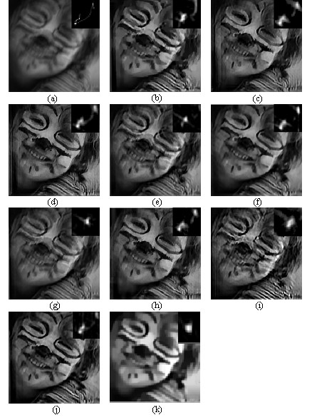
Figure 2. Deblurring Example from Levin et al. (a) Blurry Image (b) Shan et al. [12](c) Cho and Lee [14] (d) Xu and Jia [18] (e) Krishnan et al. [13](f) Levin et al. [19] (g) Pan et al. [20] (h) Xu et al. [21] (i) Zhong et al. [22](j) Dong et al. [23] (k) Our Results
Table 1. Evaluation of Levin et al. Dataset
|
Author |
References |
PSNR |
SSIM |
Time |
|
Shan et al. |
[12] |
22.69 |
0.73 |
15.53 |
|
Cho and Lee |
[14] |
23.77 |
0.75 |
2.41 |
|
Xu and Jia |
[24] |
27.45 |
0.85 |
2.82 |
|
Krishnan et al. |
[13] |
22.15 |
0.73 |
10.14 |
|
Levin et al. |
[25] |
26.46 |
0.82 |
80.59 |
|
Pan et al. |
[11] |
20.26 |
0.73 |
2.91 |
|
Xu et al. |
[17] |
27.18 |
0.86 |
2.93 |
|
Zhong et al. |
[15] |
20.48 |
0.73 |
12.61 |
|
Dong et al. |
[16] |
27.47 |
0.86 |
15.31 |
|
Y. Guo et al. |
[26] |
29.01 |
0.90 |
11.51 |
|
C.Cai et al. |
[27] |
29.83 |
0.90 |
19.31 |
|
|
Proposed Work |
30.01 |
0.91 |
18.31 |
Performance evaluation of real dataset
The proposed regularization method was also compared to state-of-the-art methods using real-world standard photos. The real-world photos lack ground truth, allowing them to be visually compared. We used techniques with their specified parameters to guarantee a fair comparison. We also utilized the Kohler et al. dataset. The dataset contained four images and each image contained twelve different blur kernels. After convolution of kernel and images, we obtained 48 different images of different sizes.
The visual findings for the Mukta image, as well as the kernels obtained by Michaeli et al. [28], Zhong et al. [15], Zuo et al. [29], Krishnan et al. [13], Jinsha et al. [30], and our LoG based, are shown in Figure 3. When compared to kernels restored by the other approaches, the visualizations of the restored kernels demonstrate the efficiency of LoG. LoG-based kernel is less sparse, and neighboring pixels are now more compressed, which can aid in the recovery of a good picture during the pre-processing step while retaining texture. Zuo et al. [29] recovered an image with a high ringing effect and enhanced the contrast of the image. Jinsha et al. [30] recovered an image that was over-smoothed because the tiny texture was ignored during image recovery. The image recovered by LoG was enhanced and it has good contouring effects.

Figure 3. Results of Mukta Image with estimated kernels (a) Krishnan et al. [13](b) Zhong et al.[15] (c) Michaeli et al. [28](d) Jinsha et al. [30](e) Zuo et al.[29] (f) LoG Based
Figure 4 depicts a visual example from Köhler et al.’s dataset [10]. The proposed method produces images that are smooth and free of ringing artifacts. We compared the results with Fergus et al. [20], Cho and Lee [14], Shan et al. [12], Hirsch et al. [31], Krishnan et al. [13], Xu and Jia [24], Xu et al. [17], Whyte et al. [32] and Dong et al. [16]. We calculated the PSNR value of this dataset. The PSNR value of our LoG based method was higher than others. The results obtained by our method are more clear.
Small local textures are preserved. The average values of PSNR and SSIM of Kohler et al.’s dataset are shown below.

Figure4. (a) Blurred (b) Fergus et al. [20](c) Cho and Lee [14](d) Shan et al. [12] (e) Hirsch et al. [31] (f) Krishnan et al. [13] (g) Xu and Jia[24] (h) Xu et al. [17] (i) Whyte et al. [32] (j) Dong et al. [16] (k)
Table II: Evaluation of Kohler et al. Dataset
|
Author |
PSNR |
|
Fergus et al. |
24.55 |
|
Cho and Lee |
33.55 |
|
Shan et al. |
28.17 |
|
Hirsch et al. |
33.12 |
|
Krishnan et al. |
25.84 |
|
Xu and jia |
32.44 |
|
Xu et al. |
35.17 |
|
Whyte et al. |
34.18 |
|
Dong et al. |
35.47 |
|
Our |
38.80 |
CONCLUSION
A Laplacian of Gaussian prior-based blind deblurring method is presented in this more efficient study. When attempting to determine the transitional latent, this approach is frequently utilized. This non-convex optimal problem that results from such a priori information is addressed by the ISTA operator. While other approaches may offer a wider range of options, using an operator provides a higher degree of precision. It is concluded that LoG can detect the edges and sharpens them. It also produces fewer ringing effects and it preserves the small local textures. It has been proven that our approach can effectively approximate the kernel and the image.
REFERENCES
[1] D. Kundur and D. Hatzinakos, "Blind image deconvolution," IEEE signal processing magazine, vol. 13, no. 3, pp. 43-64, 1996.
[2] R. L. Lagendijk and J. Biemond, "Basic methods for image restoration and identification," in The essential guide to image processing: Elsevier, 2009, pp. 323-348.
[3] J. G. Nagy, K. Palmer, and L. Perrone, "Iterative methods for image deblurring: a Matlab object-oriented approach," Numerical Algorithms, vol. 36, no. 1, pp. 73-93, 2004.
[4] J. Yuan and Z. Hu, "High-order statistical blind deconvolution of spectroscopic data with a Gauss-Newton algorithm," Applied Spectroscopy, vol. 60, no. 6, pp. 692-697, 2006.
[5] S. Sarkar, P. Dutta, and N. Roy, "A blind-deconvolution approach for chromatographic and spectroscopic peak restoration," IEEE transactions on instrumentation and measurement, vol. 47, no. 4, pp. 941-947, 1998.
[6] J. K. Kauppinen, D. J. Moffatt, H. H. Mantsch, and D. G. Cameron, "Fourier self-deconvolution: a method for resolving intrinsically overlapped bands," Applied Spectroscopy, vol. 35, no. 3, pp. 271-276, 1981.
[7] V. A. Lórenz-Fonfría and E. Padrós, "Maximum entropy deconvolution of infrared spectra: use of a novel entropy expression without sign restriction," Applied Spectroscopy, vol. 59, no. 4, pp. 474-486, 2005.
[8] L. Yan, H. Liu, S. Zhong, and H. Fang, "Semi-blind spectral deconvolution with adaptive Tikhonov regularization," Applied spectroscopy, vol. 66, no. 11, pp. 1334-1346, 2012.
[9] A. Levin, Y. Weiss, F. Durand, and W. T. Freeman, "Understanding and evaluating blind deconvolution algorithms," in 2009 IEEE Conference on Computer Vision and Pattern Recognition, 2009: IEEE, pp. 1964-1971.
[10] R. Köhler, M. Hirsch, B. Mohler, B. Schölkopf, and S. Harmeling, "Recording and playback of camera shake: Benchmarking blind deconvolution with a real-world database," in European conference on computer vision, 2012: Springer, pp. 27-40.
[11] J. Pan, Z. Hu, Z. Su, and M.-H. Yang, "$ l_0 $-regularized intensity and gradient prior for deblurring text images and beyond," IEEE transactions on pattern analysis and machine intelligence, vol. 39, no. 2, pp. 342-355, 2016.
[12] Q. Shan, J. Jia, and A. Agarwala, "High-quality motion deblurring from a single image," Acm transactions on graphics (tog), vol. 27, no. 3, pp. 1-10, 2008.
[13] D. Krishnan, T. Tay, and R. Fergus, "Blind deconvolution using a normalized sparsity measure," in CVPR 2011, 2011: IEEE, pp. 233-240.
[14] S. Cho and S. Lee, "Fast motion deblurring," in ACM SIGGRAPH Asia 2009 papers, 2009, pp. 1-8.
[15] L. Zhong, S. Cho, D. Metaxas, S. Paris, and J. Wang, "Handling noise in single image deblurring using directional filters," in Proceedings of the IEEE Conference on Computer Vision and Pattern Recognition, 2013, pp. 612-619.
[16] J. Dong, J. Pan, and Z. Su, "Blur kernel estimation via salient edges and the low rank prior for blind image deblurring," Signal Processing: Image Communication, vol. 58, pp. 134-145, 2017.
[17] L. Xu, S. Zheng, and J. Jia, "Unnatural l0 sparse representation for natural image deblurring," in Proceedings of the IEEE conference on computer vision and pattern recognition, 2013, pp. 1107-1114.
[18] A. Levin, Y. Weiss, F. Durand, and W. T. Freeman, "Understanding blind deconvolution algorithms," IEEE transactions on pattern analysis and machine intelligence, vol. 33, no. 12, pp. 2354-2367, 2011.
[19] W.-S. Lai, J.-B. Huang, Z. Hu, N. Ahuja, and M.-H. Yang, "A comparative study for single image blind deblurring," in Proceedings of the IEEE Conference on Computer Vision and Pattern Recognition, 2016, pp. 1701-1709.
[20] R. Fergus, B. Singh, A. Hertzmann, S. T. Roweis, and W. T. Freeman, "Removing camera shake from a single photograph," in ACM SIGGRAPH 2006 Papers, 2006, pp. 787-794.
[21] M. Ljubenović and M. A. Figueiredo, "Blind image deblurring using class-adapted image priors," in 2017 IEEE International Conference on Image Processing (ICIP), 2017: IEEE, pp. 490-494.
[22] L. Yang and J. Ren, "Remote sensing image restoration using estimated point spread function," in 2010 International Conference on Information, Networking, and Automation (ICINA), 2010, vol. 1: IEEE, pp. V1-48-V1-52.
[23] Y. Liao, W. Li, J. Cui, and W. Gong, "Blur kernel estimation model with combined constraints for blind image deblurring," in 2018 Digital Image Computing: Techniques and Applications (DICTA), 2018: IEEE, pp. 1-8.
[24] L. Xu and J. Jia, "Two-phase kernel estimation for robust motion deblurring," in European conference on computer vision, 2010: Springer, pp. 157-170.
[25] A. Levin, Y. Weiss, F. Durand, and W. T. Freeman, "Efficient marginal likelihood optimization in blind deconvolution," in CVPR 2011, 2011: IEEE, pp. 2657-2664.
[26] Y. Guo and H. Ma, "Image blind deblurring using an adaptive patch prior," Tsinghua Science and Technology, vol. 24, no. 2, pp. 238-248, 2018.
[27] C. Cai, H. Meng, and Q. Zhu, "Blind deconvolution for image deblurring based on edge enhancement and noise suppression," IEEE Access, vol. 6, pp. 58710-58718, 2018.
[28] T. Michaeli and M. Irani, "Blind deblurring using internal patch recurrence," in European conference on computer vision, 2014: Springer, pp. 783-798.
[29] W. Zuo, D. Ren, D. Zhang, S. Gu, and L. Zhang, "Learning iteration-wise generalized shrinkage–thresholding operators for blind deconvolution," IEEE Transactions on Image Processing, vol. 25, no. 4, pp. 1751-1764, 2016.
[30] J. Pan, D. Sun, H. Pfister, and M.-H. Yang, "Blind image deblurring using dark channel prior," in Proceedings of the IEEE Conference on Computer Vision and Pattern Recognition, 2016, pp. 1628-1636.
[31] M. Hirsch, C. J. Schuler, S. Harmeling, and B. Schölkopf, "Fast removal of non-uniform camera shake," in 2011 International Conference on Computer Vision, 2011: IEEE, pp. 463-470.
[32] O. Whyte, J. Sivic, A. Zisserman, and J. Ponce, "Non-uniform deblurring for shaken images," International Journal of computer vision, vol. 98, no. 2, pp. 168-186, 2012.
 |
Copyright © by authors and 50Sea. This work is licensed under Creative Commons Attribution 4.0 International License.
|