EVALUATING FOCAL MECHANISM OF SEPTEMBER 24, 2013 AWARAN EARTHQUAKE WITH GEOSPATIAL TECHNIQUES

Israr Ahmad1, RanaWaqarAslam1,5*, Lin Li2, Muhammad Burhan Khalid3, Waqas Abbas3, Aqsa Aziz4, Muhammad Nassar Ahmad1, Ali Imam Mirza5, Ali Iqtadar Mirza5

1State Key Laboratory of Information Engineering in Surveying, Mapping and Remote Sensing (LIESMARS), Wuhan University, Wuhan 430079, China.

2School of Resource and Environmental Science), Wuhan University, Wuhan 430079, China.

3 Punjab University College of Information & Technology, University of the Punjab, Lahore.

4Department of Geography, University of Punjab, Lahore. 5Department of Geography, Government College University, Lahore.

*Corresponding Author’s Rana Waqar Aslam Email: ranawaqaraslam@whu.edu.cn.

Citation |Ahmad. I, Waqar. A, et al., “EVALUATING FOCAL MECHANISM OF SEPTEMBER 24, 2013 AWARAN EARTHQUAKE WITH GEOSPATIAL TECHNIQUES”. International Journal of Innovations in Science & Technology, Vol 02 Issue 03: pp 108-124, 2020.

Received |Aug 20, 2020; Revised | Sep 15, 2020; Accepted | Sep 18, 2020; Published | Sep 20, 2020 ________________________________________________________________________

Abstract.

Seismic records from IRIS (NIL, KBL, MSEY, KMI, QIZ, DGAR) were used to compute AWARAN September 24 2013 Earthquake's focal mechanism. Earthquakes are one of the most drastic threats that are likely to cause heavy human casualties and can destroy entire cities within minutes. We processed the waveform data from 6 separate stations for the computation of displacement. The issues related to attenuation have been overcome by the use of low frequencies (0.05-0.1). The crustacean model that determines the tensor PREM model's time is determined by minimizing the variance but produces a robust focal mechanism. Inverting the displacement data is applied to recover the moment tensor from the source, calculated the green feature with the reversal. GIS-based vectors of fault lines were abstracted by the digitization of regional tectonic lineaments and structural maps. We developed synthetic and observed surface shapes with a 100 percent dc correlation. Our understanding of the features of crustacean deformation and regional tectonics in the area will benefit from the resulting focus mechanisms. The measured earthquake focal mechanism is similar to a USGS agency hit, dip, and rake.

Keywords: Awaran earthquake, Focal Mechanism, PREM Model, Green Function, GIS.

Introduction

Seismic tremor or earthquakes are natural hazards which devastate the natural beauty and ecological balance of a region badly, [1]. The earthquake in AWARAN on September 24, 2013, was triggered by an oblique landslide movement in one of Chaman 's southern strands, [2]. The event took place within the large area of the plate limit established by the Makran Cumulative Prism and the Chaman Fault System, [3]. It was situated in a region with well defined fault morphologies, [4 ][5 ]. but large (>M7) historical earthquakes were not previously observed, [ 6 ][ 7 ].The surface crust depth (15 to 20 km), the northern slip movement and the internal depth was approx. 80 km as shown [8]. In 1935, the Mw 7.5 earthquake occurred at the Ghzaband fault, [9]. The core mechanisms of medium-depth earthquakes have been clarified mainly in response to the decreasing extension in many subduction areas worldwide, [10]. Seismic procedures provide the highest accuracy of the earth's internal structure than any geophysical method, [11]. This is because elastic waves of any geophysical wave have the shortest wavelength and because the physics which regulates their spatial and temporal sensitivity determines the origin of energy, [12][13]. Several methods for evaluation of point-source and source-time (STF) process for events were established simultaneously, [14]. The use of waveform modelling for calculating focus mechanisms depends on modern tools [15][16][17]. The tensors depend on the spring strength and fault path [18]. The pivoting function or the solving of problems of the plane also implies "beach balls." It gives us a feeling about seismic waves that originate from a complex rupture, involving space and time displacements that are abnormal [19]. Furthermore, it is a plus point to write that is any orthogonal coordinate system since vector and tensor equations are valid irrespective of the coordinates of system. Ordinary data reversal techniques [20] surface waves [21][22][23] and body waves [24][25] have been evaluated and the reversal of broadband seismic charts has been proposed for regional earthquakes [26]. Other methods are also used to evaluate influential movement records and the depth of the source [27]. 

The ISOLA Interface is used for instance, which carry out certain tasks to access all investment procedures, [28] [29]. The green function is measured by wave frequency method, [31] [32]. The code is written in Fortran, but the user can control its use through ISOLA-GUI, [33]. ISOLA-GUI creates all the required files with the inspection diagrams (Descartes and Geographies coordinates) for calculating the Green-Inversion function, [34] [35]. The relationship representing the percentage of a double pair solution is defined, since it can show problem output in investment. The modules run concurrently and most of them "know" the answer from the user or try to suggest acceptable processing parameters. Significant information on regional and local tectonics is given for medium sized earthquakes in the country, [36]. The focusing mechanisms calculated using only the first direction of movement can thus have a significant effect on the parameters of the coordinating mechanism calculated by these incorrect measurements of the first movement. Depending upon the distribution and consistency of the first motion data, more than one focus mechanism fits to the data. The key benefit of the instantaneous tensor is that seismographs can be reversed to identify the source parameters. Instant tensors for reflection are defined as the movement of an error during an earthquake consisting of nine pairs or nine sets of two vectors.

Material and Methods.

Investigation site.

There were many earthquakes, mostly occurred in coastal areas in Balochistan. District of Awaran is situated (Fig. 1) in the south of the province of Baluchistan (Lat: 27,016 ° N; 65,547 ° E). The red zone for earthquakes in Pakistan is known to be the Mekran range due to tectonic activities. In the remote and inaccessible regions, the earthquake caused widespread destruction and the death toll reached over 825 . Awaran, Ritaj, Jashkur, Nok Jo, Parwar, Dandar and Hoshab were the affected areas. Almost 33,000 homes and 300,000 individuals suffered from the earthquake, [37]. . The Awaran earthquake was caused by the southern strands of the Hoshab fault in the Chaman fault system. An analysis of high-resolution World View 2 satellite images also confirms the rupture on the left side of the surface. Another confirmation was made of Landsat-8 image for the rupture that corresponded to the Hoshab failure. The event ruptured the Makran subduction megathrust. The earthquake was 7.7 as measured on the Richter scale. A new island formed called “mud volcano” on the sea floor following the earthquake. The epicenter was situated in an area influenced by the above two crash logics. A complex collection of mountains folding and fissured along the coast and northbound to the west from India and Eurasia's convergence area resulted from relative closeness between the two species [38].

Figure 1. Location of Awaran earthquake September 24th, 2013
Awaran Earthquake in Terms of Richter Scale
Charles F. Richter developed the Richter Scale in 1935. Originally, the earthquake was 7.4 MW and then upgraded to 7.8 but later changed to 7.7, on the Richter scale. A heavy shaking (VII) occurred in the nearby town of Awaran on the 24th September, with a major shaking in the big town of Kharan and a heavy shaking in Hyderabad and mild shaking in Karachi.

Table 1. Details of September 24 earthquake

Makran tectonic map is shown in the figure 2.

Figure 2. There are major faults on the tectonic map of southern Pakistan.

A full black circle is the core location of the Awaran earthquake [18] It spreads over 400 km north and a 1000 km east, and can subducts under the Eurosian platform by 3 cm / year north of the Arab plate and Ormara.. In 1945, an 8.0 MW earthquake broke the enormous Makran thrust. The Chaman fault system is a 1200 km lefthand failure system adjusted for 3 cm / yr north of India in relation to Eurasia. The Chaman fault system consists of the Ornach Nal, Ghazaband and Chaman 's sinister failures. In the south, the Chaman defects refer to the Seyhan, Punjur and Hushab Makran chains' defections and those defections are internalised; the tale from India and Eurasia and the shorter one from the Arab Peninsula and Eurasia. The faults left in the side blow sliding faults of the Chaman and Urnash-Nal power the Indians and Eurasians' crash. Landslide systems predominantly form the Makran subduction zone boundaries. The fault system Ornach-Nal marks the eastern frontier, while the fault system Minab-Zendan represents the western border. As the Arabian plate is compressed, in the Makran area and the Chagai Arc, there is a directional tendency between east and west. It implants with an implantation angle of 2-8 degrees at a speed of 19.5 mm per year.  

Figure 3. 2013 Earthquake in MW 7.7 Awaran. (a) An aerial view of the Oran area's destruction. (b) A view of the island following an earthquake in Awaran [8]

In Ziarat, the 1.300 Kilometers long Hass Soliman fracture, the Chaman fault and the Sibi basin are regulated by the tectonic and structural patterns. Quetta's local defect structures are comprised of Chaman 's Fault, Chengin Gulat structure, Harnai Tarta Structure, Gzband Gob Chassis, and Mach Chassis. The Makran Coast Fault is 225 km long in south of Ormara and Pasni. The earthquake occurred in the depth of the ground crust over the Makran subduction zone as a result of oblique displacement. The study is based on the seismic waveforms data which is available at https://ds.iris.edu/ds/nodes/dmc/data/types/waveform-data/ that was recorded at different stations of the world in response to the earthquake that struck just near the district Awaran on September 24, 2013.
Table 4. Stations Information of September 24, 2013, AWARAN earthquake

For proper coverage of Awaran earthquake, we set the distance from 0 to 180 degrees using powered. The coverage to the event was ensured from all sides for a better display of results. The start and end time are adjusted such that complete waveforms are obtained. A total 6 IRIS stations for Awaran earthquake were selected such that a proper coverage to the earthquake epicenter was ensured. Our goal was to measure the tensor moment. The first-order seismic tensor is an extensive representation of earthquake sources resulting in a straightforward linear relation with a sequence of green and fundamental error reactions. . So, we choose the station for which waveform data was available for all N, E, Z and time components.

Figure 4. In the figure the orange circle shows the location of September 24th,2013 Awaran earthquake epicentre, While the red triangle shows the location of the recording NIL station (located in Nilore Isl amabad

Figure 5. Flow chart of Methodology Adopted for the work Defining Proper Crustal Model for Earth
ISOLA-GUI operation is a crustal model built with the crustmod tool for all subsequent analysis steps (for example, green function measurement, polarity control, etc.). The vector speeds (Vp and V), density, P and S (Qp and Q) are inserted either in text boxes or in text files when the Matlab code provides correct formatting for ISOLA fortran coding. Some devices were available with experimental relationships for generating Vp and V velocity graphs with depth and measurement of V and strength. For each season, the symbol supports one cortical model, but future releases support several cortical models. We used the PREM Crustal model to calculate the current tensor for the study period. The main reference earth model (PREM) was 1-D used for seismic experiments on the planet for several yearsThis model has been developed for various data sets, including free centre oscillation frequency measurements, monitoring of surface waves scattering, travel times for different phases of body waves, radio astronomical data from the field, mass and moment of tranquilly. For our study area, we used 12 layers of the earth's surface (depth 0) to the inner core (6371 km).

Figure 6. In this PREM Model above the red line shows Vs (Shear wave velocity) and blue line sho ws the Vp (Primary wave velocity). We notice that from 3000 - 5200 the Shear wave velocity (Vs) value obtained is zero. Green Functions Computation
The green function is computed using the waven number method. Like coupon delivery, several codes are available remotely to represent data in bullet source or multiple instantaneous tension models. Fortran codes exist as separate executable files called ISOLAGUI for tasks such as computing and Green reversal. For additional M5 + earthquakes at distances up to 400 km, the code is also proven useful. The overall frequency for our work to measure the green function was 0.1. It was crucial for our results to use such a low frequency in our work, because the attenuation of such lower frequency is not very important. Therefore, the attenuation issue largely doesn't affect our performance. Spatial Analysis The primary data of earthquakes was accessed from open source earthquake databases of US Geological Survey and Pakistan Seismic Network of Pakistan Metrological Department.The dataset of 4031 events (spreading over 7 ºN to 32º N and 55º E to 71º E) has been self-reviewed and annotated for cataloging. The magnitudes of those events were measured in different scales ranging between 3.7 <m< 8.1. All kinds of magnitude scales have been translated into unified magnitude scale i.e. moment magnitude (Mw) which is considered most reliable magnitude scale for cataloging. The capabilities of ArcMap tools have been explored for data analysis, clipping and mapping of desired earthquake data. The clipping tools of ArcMap were utilized to select the events within the buffer around a fault line and tectonic lineaments. The clipping tool improve the efficiency in getting data points in response of spatial queries. Since, the primary key of earthquake dataset is the spatial coordinates of epicentre of each event.

Figure 7. History of Earthquakes from 1900 to 2016
Result and discussion. This research involves calculating the location and frequency of reflection of the waveform for a test depth in the horizontal source (in the SED position, i.e. in the USGS Focus centre). Fortran ISOLA code is used to revert the Waveform to use speed, while the user interacts even during reflecting in the Mat lab environment. The broad slip of a young failure and an active failure is a riddle about fault geometry's supposed impact on failure dynamics. The seismically active error plans tend to be optimally directed to Anderson's error theory. Slip or slip sources often come out from the axial mechanism of low-cross earthquakes, but slip slipping is relatively rare.. In Fig.8, which shows the stability of the focal length and the best acceptable depth at 17.5 km, the connexion between observations and artificial seismograms is shown in terms of depth. The maximum correlation was found at 0,43 at a depth of 17,5 km and the CC is 100% double. Baluchistan’s earthquake highlighted the engineering flaws, preconfigured stress and dynamic vulnerability, as was the case on several previous occasions on the seismic breakage propagation from dynamic modelling.

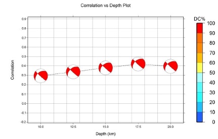
Figure 8. As a function of the test source deepness down the SED focus centre, the correlation between the ob served, artificial and focal mechanism waves. DC percent of colors We determined the earthquake focal mechanism, which equates the USGS strike, sinking and tilt. Then we reverse the seismogram in order to measure the time of launch, the intensity of the earthquake and the tensor's six components. Figures 9 and 10 demonstrate the effects of the reflection. Seismic moment was observed approximately 4,037e + 20 Nm, the equivalent of Mw 7,7. US Geological Survey has reported the same scale. In contrast to a depth of 15.5 km, the best approach was measured at a depth of 17.5 km. The synthetic seismograms, as shown in the figure, well suit the observations.

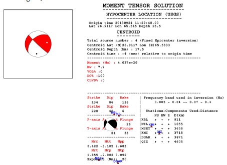
Figure 9. Moment tensor solution of the Awaran earthquake. Triangles show the station used in the inversion.

Figure 10. Observed (green line) and synthetic (blue line) velocity (m/s): Frequency ranges 0.005 – 0.1 Hz, Event 1. Peak amplitudes (in m/s) are on the right - hand side of the figure Since the occurrence of event, the times (in second) are given on the bottom of the plot Cross-section of Slip Distribution
The strike direction is indicated above each fault plane and the hypocenter location is denoted by a star. Slip amplitude is shown in color and the motion direction of the hanging wall relative to the footwall (rake angle) is indicated with arrows. Contours show the rupture initiation time in seconds.

Figure 11. Cross - section of Slip Distribution

Surface projection
Surface projection of the slip distribution was superimposed on GEBCO bathymetry. Thick white lines indicate major plate boundaries [Bird, 2003]. Gray circles, if present, are aftershock locations, sized by magnitude.

Figure 12. Surface Projection
Spatial analysis of Epicentres of magnitudes
The study area is seismically active, it is diversified in seismogenic potential, earthquake born processes, and consequential variation in magnitude strengths of the earthquakes. The magnitude of earthquakes quantifies the amount of elastic strain energy released during the earthquake. It was revealed that the changes in magnitude strength are not just the statistical data variations, but these changes are closely articulated with the seismo-geological characteristics, deformation and depth of the active fault segments, microseismic proximity to the active margins, structural stability, fault mechanics and its kinematics etc.

Figure 13. (a)Seismic map of Pakistan                         Figure 13. ( b ) Shakemap of Pakistan

Tectonic Summary
The Awaran earthquake of magnitude, M 7.7 earthquake in south-central Pakistan occurred as a result of oblique strike-slip type at shallow crustal depths. The location, focal mechanism solutions, and finite-fault modeling of the earthquake are consistent with leftlateral (southwest-striking) rupture within the Eurasia plate above the Makran subduction zone. The event occurred within the transition zone between northward subduction of the Arabia plate beneath the Eurasia plate and northward collision of the India plate with the Eurasia plate. The epicenter of the event is 69 km north of Awaran, Pakistan, and in 270 km north of Karachi. On a broad scale, the tectonics of southern and central Pakistan reflect a complex plate boundary where the Indian plate slides northward relative to the Eurasian plate in the east, and the Arabia plate subducts northward beneath the Eurasia plate in the Makran (western Pakistan). These motions typically result in north-south to northeastsouthwest strike-slip motion at the location of the September 24th earthquake that is primarily accommodated on the Chaman fault, with the earthquake potentially occurring on one of the southernmost strands of this fault system.

Figure 14. Tectonic map of Pakistan
While commonly plotted as points on maps, earthquakes of this size are more appropriately described as slip over a larger fault area. Strike-slip events are typically about 160x20 km (length x width). Modelling of this earthquake implies dimensions of about 200x20 km, predominantly up-dip and southwest of the hypocentre. Although seismically active, this portion of the Eurasia plate boundary region has not experienced large damaging earthquakes in the recent history.
Conclusion
The data from 6 stations (NIL, KBL, MSEY, KMI, QIZ, DGAR) was used to compute focal mechanisms. By using the low frequencies (0.05-0.1), the problems arising due to attenuation were significantly reduced. The maximum correlation was noticed at 0,43 at a depth of 17,5 km where the CC was 100% double. Baluchistan’s earthquake highlighted the engineering flaws, preconfigured stress and dynamic vulnerability, as it was the case on several previous occasions on the seismic breakage propagation from dynamic modelling. The plot of observed waveforms versus synthetic waveforms is well correlated. The use of a standard ground model such as PREM provided a robust focal mechanism. The Mat labbased graphical user interface makes data management easy, while offering full user control in the workflow and an intuitive graphical overview of the findings. The quantity of DC (double pair) was estimated as 7,7 100%. Today Pakistan is a seismically active and vulnerable to major seismic events. In Pakistan, tectonics needs to be re-invested as a matter of urgency and secret defects found in areas where the population is seriously endangered.

Acknowledgment. The authors would like to thanks the anonymous reviewers for their hard work. IRIS, Berkeley University of California and the Institute of Technology have provided the seismic data used. Open access to these data enables and is widely valued.

Source of Parkfield seismic data: U.S. Geological Survey. Author’s Contribution. All authors have contributed equally.

Conflict of interest. The authors declare no conflict of interest in publishing this manuscript in IJIST.

REFERENCES

1. Saifullah.M, Asghar. A, Ahmad.A.M, Zafar.M, Saman.S, Arshad A.M, Akhtar.A. “Computation of Temporal Decline to a Vanished Island (A Case Study Zalzala Koh)”. International Journal of Innovations in Science & Technology, Vol 01 Issue 04: pp 142150, 2019.

2. Ambraseys, Nicholas, and Roger Bilham. “Earthquakes in Afghanistan , Seismological Research Letters, Vol 74 issue 2, pp: 107–23, 2002

3. Aochi, Hideo, Raul Madariaga, and Eiichi Fukuyama. “Constraint of Fault Parameters Inferred from Nonplanar Fault Modeling.” Geochemistry, Geophysics, Geosystems, vol 4 issue 2 pp: 1–16. 2003.

4 Avouac, Jean Philippe et al. “The 2005, Mw 7.6 Kashmir Earthquake: Sub-Pixel Correlation of ASTER Images and Seismic Waveforms Analysis.” Earth and Planetary Science Letters, Vol 249, issue 3–4, pp: 514–28, 2006.

5 Barnhart, W. D. et al. “Evidence for Slip Partitioning and Bimodal Slip Behavior on a Single Fault: Surface Slip Characteristics of the 2013 Mw7.7 Balochistan, Pakistan Earthquake.” Earth and Planetary Science Letters , Vol 420, issue 12, pp: 1–11, 2015.

6 Bilham, Roger et al. “Seismic hazard in Karachi, Pakistan: Uncertain past, uncertain future” Seismological Research Letters , Vol 78, issue 6, pp: 601–13, 2007.

7 Bormann, Peter. “Global 1-D Earth Models 1 PREM Model.” Datasheet, Vol 1, issue 1, pp : 1–12, 2002.

8 Bouchon, Michel. “The Discrete Wave Number Formulation of Boundary Integral Equations and Boundary Element Methods: A Review with Applications to the Simulation of Seismic Wave Propagation in Complex Geological Structures.” Pure and Applied Geophysics, Vol 148, issue1–2, pp : 3–20, 1996.

9 Buforn, E., C. Sanz de Galdeano, and A. Udías. “Seismotectonics of the IberoMaghrebian Region.” Tectonophysics , Vol 248, issue 3–4, pp: 247–61, 1995.

10 Buland, Ray, and Freeman Gilbert. “Matched filtering for the seismic moment tensors.” Geophysics research letter, Vol 3, issue 3, pp: 205–206, 1976.

11 Celerier, Bernard. “Seeking Anderson’s Faulting in Seismicity: A Centennial Celebration.” Reviews of Geophysics (2007), Vol 46, issue 4, pp: 1–34, 2008.

12 Dziewonski, Adam M. “Preliminary Reference Earth Model,” Physics of Earth Planet. Intereriors, Vol 25, issue 4, pp: 297–356, 1981.

13 Frohling, E., and W. Szeliga. “GPS Constraints on Interplate Locking within the Makran Subduction Zone.” Geophysical Journal International, Vol 205, issue 1, pp: 67–76, 2016.

14 Isacks, Bryan, and Peter Molnar. “Correction [to ‘Distribution of Stresses in the Descending Lithosphere from a Global Survey of Focal‐mechanism Solutions of Mantle Earthquakes’].” Reviews of Geophysics Vol 10, issue 3, pp: 847–847, 1972.

15 Kanamori, Hiroo, and Jeffrey W Given. “Use of long-period surface waves for rapid determination Of Earthquake-Source Parameters.” Physics of Earth Planet. Intereriors,Vol 27, issue 1, pp: 8–31, 1981.

16 Kikuchi, M, and H Kanamori. “Note on Teleseismic Body-Wave Inversion Program” Earthquake Research Institute, Tokyo University, Japan, pp: 2335–50, 2003. 17 Lawrence, R. D. et al. “Thrust and Strike Slip Fault Interaction along the Chaman Transform Zone, Pakistan.” Geological Society Special Publication Vol 9, issue 1, pp: 363–70, 1981.

18 Mahmood, Irfan. “Revisiting major earthquakes in Pakistan.” Geology today.Vol 31, issue 1, pp: 33–38, 2015.

19 McCaffrey, Robert. “Earthquakes and Ophiolite Emplacement in the Molucca Sea Collision Zone, Indonesia.” Tectonics, Vol 10, issue 2, pp: 433–53, 1991.

21 Mokhtari, Mohammad, Ahmad Ala Amjadi, Leila Mahshadnia, and Mandana Rafizadeh. “A Review of the Seismotectonics of the Makran Subduction Zone as a Baseline for Tsunami Hazard Assessments.” Geoscience Letters, Vol 6, issue 1, pp: 1–9, 2019.

22 MonaLisa, and M. Qasim Jan. “Awaran, Pakistan, Earthquake of Mw 7.7 in Makran Accretionary Zone, September 24 2013: Preliminary Seismotectonic Investigations.” Proceedings of the Pakistan Academy of Sciences, Vol 52, issue 2, pp: 159–68, 2015.

24 Oglesby, D. D., and S. M. Day. “Fault Geometry and the Dynamics of the 1999 ChiChi, (Taiwan) Earthquake.” Bulletin of the Seismological Society of America, Vol 91, issue 5, pp : 1099–1111, 2001.

26 Patton, Howard. “Determination of Seismic Moment Tensor Using Surface Waves.” Tectonophysics, Vol 49, issue 3-4, pp: 213–22, 1978.

27 Platt, J. P., J. K. Leggett, and S. Alam. “Slip Vectors and Fault Mechanics in the Makran Accretionary Wedge, Southwest Pakistan.” Journal of Geophysical Research Vol 93, issue 137, pp: 7955–73, 1988.

28 Quittmeyer, R.C., and K.H. Jacob. “Historical and Modern Seismicity of Pakistan, Afghanistan, Northwestern India, and Southeastern Iran.” Bulletin of the Seismological Society of America, Vol 69, issue 3, pp: 773-823, 1979.

29 Reilinger, Robert et al. “GPS Constraints on Continental Deformation in the AfricaArabia-Eurasia Continental Collision Zone and Implications for the Dynamics of Plate Interactions.” Journal of Geophysical Research: Solid Earth, Vol 111, issue 5, pp: 1–26, 2006.

30 Ritsema, J., and T. Lay. “Long-Period Regional Wave Moment Tensor Inversion for Earthquakes in the Western United States.” Journal of Geophysical Research, Vol 100, issue 1, pp: 9853-9864, 1995.

31 Sekiguchi, Haruko, Tomotaka Iwata, and Izmit Bay. “Rupture Process of the 1999 Kocaeli , Turkey , Earthquake Estimated from Strong-Motion Waveforms.” (February) , Volume 92, issue 1, pp: 300–311, 2002.

32 Sipkin, Stuart A. “Estimation of Earthquake Source Parameters by the Inversion of Waveform Data: Synthetic Waveforms.” Physics of Earth and planetary interiors, Vol 30, issue 2-3, pp: 242–59, 1982.

33 Sokos, Efthimios N., and Jiri Zahradnik. “ISOLA a Fortran Code and a Matlab GUI to Perform Multiple-Point Source Inversion of Seismic Data.” Computers and Geosciences, Vol 34, issue 8, pp: 967–77, 2008.

34 Stich, Daniel, Charles J. Ammon, and Jose Morales. “Moment Tensor Solutions for Small and Moderate Earthquakes in the Ibero-Maghreb Region.” Journal of Geophysical Research: Solid Earth Vol 108, issue B3, pp: 1-4, 2003.

35 Vernant, Ph et al. “Present-Day Crustal Deformation and Plate Kinematics in the Middle East Constrained by GPS Measurements in Iran and Northern Oman.” Geophysical Journal International Vol 157, issue 1 pp : 381–98, 2004.

36 Wessel, Paul, and Walter H.F. Smith. “Free Software Helps Map and Display Data.” Eos, Transactions American Geophysical Union Vol 72, issue 41, pp : 441–46, 1991.

38 Wiedicke, M., S. Neben, and V. Spiess. “Mud Volcanoes at the Front of the Makran Accretionary Complex, Pakistan.” Marine Geology, Vol 172, issue 1–2, pp: 57–73, 2001.