Evaluating Artificial Intelligence and Statistical Methods for Electric Load Forecasting

Usman Dilawar¹, Abdul Khaliq², Nadeem Kureshi³

^1,2,3 Department of Electrical & Computer Engineering, Sir Syed CASE Institute of Technology,  Islamabad, Pakistan

* Correspondence: Usman Dilawar , mud.sscaseit@gmail.com.

Citation | Dilawar. U, Khaliq. A and Kureshi. N, “Evaluating Artificial Intelligence and Statistical Methods for Electric Load Forcasting”. International Journal of Innovations in Science and Technology”. Vol 3, Special Issue, pp: 59-83, 2022

Received | Dec 14, 2021; Revised | Dec 19, 2021 Accepted | Dec 27, 2021; Published | Jan 1, 2022.

________________________________________________________________________Abstract.

Electric Load Forecasting (ELF) is one of the challenges being faced by the Power System industry. With the ever-growing consumer demand, power generating companies struggle to manage and provide an uninterrupted power supply to the users. Over the past few decades, the introduction of smart grids and power deregulation has changed load forecasting dynamics. Most of the current research focuses on short-term load forecasting (STLF), involving an hour to a week’s time forecasting. Various techniques are being used for accurately predicting the electric load. However, gold standards are yet to be defined mainly because of the subject's variety, non-linearity, and un-predictive form. In this study critical review of 25 publications has been carried out to find the most efficient method for ELF. The novelty of this study is that comparative and scientific analyses are carried out to find the most proficient techniques for load forecasting.  Also, various parameters are combined for comparison in this study after analyzing published reviews on the subject. Artificial Neural Networks (ANN) and Auto-Regressive Moving Average (ARMA) models outperform other methods basing upon statistical analysis, i.e., Mean Absolute Percentage Error (MAPE) and comparative acceptance, in the research community.

Keywords: Electric load forecasting, Power load, Modelling electricity loads, Long term/ Short term forecasting, Performance management. 

Introduction

Electric Load Forecasting (ELF) has been a prime area of concern since the advent of electricity. Predicting future load helps power utility companies to plan and meet the power generation with consumer’s demands. ELF is also one of the significant factors for regulatory bodies, industries, trading and insurance companies [1]. With technological advancement, the integration of smart devices in various technical fields has become a norm, and the power industry is not an exception. Additionally, due to global warming issues, inclination towards renewable energies resulted in the introduction of smart equipment in power generation and grid systems. The same has resulted in the availability of digitized data, which on the other hand, became helpful for analysis and future prediction [2]. The consumer’s electricity demand is increasing day by day, as the world has moved towards an automated version of almost everything. Traditional power generating companies face challenges to meet user demands, and their return on investments are declining. A strong change in the power sector is observed during the 1990s with deregulation and market competition [3]. On the other hand development of smart electronics devices has gained popularity in generating power more efficiently. The volatility of electricity is adamant with the fact that it has to be provided promptly. A huge amount of electricity cannot be stored; hence equating generation with the user demands is a tough task. ELF has thus emerged as a vibrant field for the scientific community. An accurate load prediction enables decision-making by the power operators. The power industry thus invested a lot in this field to compete in the market and avoid burning extra fuel or running machinery to generate abundant electricity.

ELF is generally categorized in long, medium, and short-term forecasting on a temporal basis. Though no standard categorization has been laid so far, all of them are interconnected in the broader perspective. Long Term Load Forecasting (LTLF) – spand the load prediction for three years or more. For less than three year time period, it is termed medium forecasting (MTLF). Finally, forecasting is carried out in the short term (STLF) from an hour/ half-hour to a week’s time [1]. With the growing renewable power generation systems, the introduction of smart grid systems, and privatizations, short-term and very short-term forecasting have gained popularity. This study is aimed to review published literature to look for the best technique for electric load forecasting. Rest of this paper is divided into four major postions. In the first, literature review is carried ou following the explanation of research methodology applied in this study. Findings with comparative analysis and results are explained in the next part. Finally, the discussion is carried out before concluding the study.

Literature Review

Calculation of load is one of the significant factors for power companies. All the operations and planning of power generation, transmission, maintenance, etc., are based on future load value. The forecasting helps in decision making as well as reducing the risk of non-availability of power. Several conventional methods of forecasting are already in practice. Over the period, various techniques have been researched to improve load forecasting.

The qualitative methods forecast are based upon the opinions and discussion with domain experts. These methods are employed when historical data is not available for a forthcoming event. Estimates are generally vague and can lead to a blackout. The Quantitative techniques involve Time Series Analysis and Econometric Analysis. A variable of interest is defined in time series such that its value is estimated relying on the relevant historical data. Baseband model, Trend model, Linear Regression models are few examples. The econometric analysis considers the drivers such as business index, weather index, etc. such that they further leads to estimate demand requirements. Recently, Artificial Intelligence (AI) has out-performed the conventional methods in the fields where non-linear and complex data is involved. The non-linear demands, transmission losses, climate factors, etc., and their relationships have made load forecasting a potential field for application of AI techniques. Artificial Neural Networks (ANN), Support Vector Machines (SVM), Genetic Algorithm, Fuzzy Logic, Self-Organizing Maps, Extreme Learning Machines are few AI techniques that can be employed in load forecasting. Various reviews and analyses done on the subject are consulted to develop a comprehensive meta-analysis approach for this study. Table 1 depicts the methods followed by previously published studies on the subject.

Table 1.  Previous Reviews on ELF

Reference Review	Method
[1]	Commonly used by Expert Community
[4]
[5]	MAPE Percentages
[6]
[7]	RMSE Percentages
[8]	Data and Error measured (MAPE, RMSE)

The main contributions of this paper are:

• Results are generated based on a comparative and statistical analysis of different studies already published in the subject field. Since both analyses have different implications. Comparative analysis shows the acceptance of different techniques in the research community. While on the other hand, the statistical analysis compares results in mathematical form.
• Previous reviews on ELF are first analyzed to select the parameters to compare various studies on the subject further.
• A systematic review is carried out for considering the studies published in various journals. The aim is to cover the subject domain in a wholesome and diverse manner.
• The research community can benefit by realizing the theoretical and statistical performance of various methods from this study.

Research Approach

Research is an ongoing process where methods and theories are developed and supported by logic and proof. Its main objective is to combine published methods and theories of one category and compare them with that of another in a systematic manner to reach some conclusion [9]. Meta-analysis is a common field of almost all research disciplines. It consists of five basic steps involving finding relevant studies on the subject, developing consistent criteria for comparison, recording relevant information from the study as per the criteria, analyzing information to compile them in broad contours, and finally drawing conclusions basing upon these findings [10]. This study aims to review the academic literature to explore the most efficient methods being used for STLF. Critical analysis is carried out to analyze the dynamics and performance of various methods and techniques employed.

The general framework of this study comprises two phases. In the first phase, research papers and articles are searched in most databases on the internet centered upon specific keywords. In the next phase, developed methods and their results are analyzed statistically. The general framework of this research is shown in Figure 1.

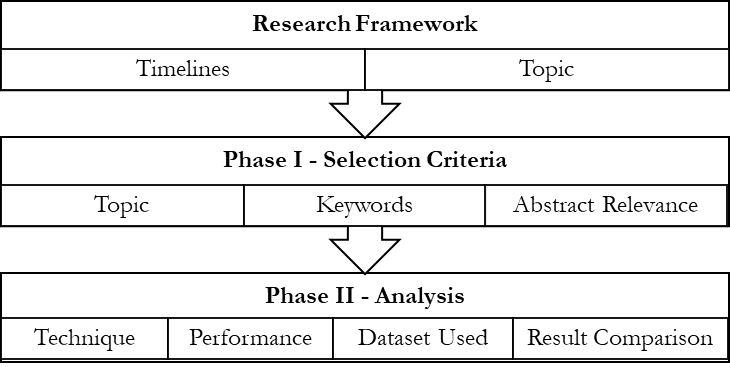
Figure 1. General Framework.

Research Catalogue

In phase I, to systematically review the literature, search is mainly carried out from 2000-2020 by using specific keywords and search engines. Scopus and IEEE Xplore are the most reliable databases in the scientific community. Both these databases are used with the keywords “electric load forecasting,” “power load,” “modeling electricity loads,” and “long term/ Short term forecasting.” Eight thousand five hundred five papers and articles came out due to search initially, including papers from areas of computing, power market, and wind energy. The advanced research tool is used to narrow down the search to a specific area of power engineering, resulting in 5,009 papers. The search is further refined based upon the title of the papers to locate 1865 papers relevant to electric load forecasting and STLF. Keeping in view the time constraint, the scope of the project, and resources available, 25 papers on STLF are selected for review and meta-analysis purposes. The topmost journals that contributed towards the selected topics are found to be IEEE Transactions on Power Systems, IEEE Transactions on Power Grids, International Journal of Forecasters, and International Journal of Electrical Power and Energy System, as shown in Graph 1.

Graph 1. Journal Wise Publications.

Analysis Approach.

Finally, in phase II, each publication is studied in detail for comparative analysis after selecting publications during the initial phase. Owing to the variability of consumer’s load demands due to various meteorological conditions, socio-economic conditions, a two-pronged approach is applied in this study. Firstly, specific criteria are developed to analyze and compare the studies in detail. Since each step of the research contributes to the studies' final results, criteria are developed in such a sense that it covers complete research methodology. Secondly, the proposed methods are compared for statistical analysis as per their Mean Absolute Percentage Error (MAPE) results. This study assumes that all the results published in the studies are correct, methods used by the majority of the expert community are best, and finally, MAPE percentages of the studies are compared.

Criteria of Analysis.

Different performance measures and results are used in different papers as per their requirements. However, meaningful meta-analysis can only be done based on some criteria. This criterion needs to be selected very thoughtfully. If it misses the relevant parameters of the respective research theme, then the chances are high that meta-analysis may not make correct assessments. Henceforth, various systematic literature reviews and studies on the subject are consulted before defining comparison criteria for this study. Criteria given in Table 2 are used to compare the papers in this study.

Table 2. Criteria for Analysis of Various Studies.

Category	Description
Proposed Method	Essence of this study, as we want to check which methods used for STLF are more reliable and efficient.
Dataset Used	Number of samples or data used as input plays critical role in estimation.
Overview of the Methodology	What methodology is used by the author Long/ Medium/ Short/ Very Short Term Forecasting
Performance Measure	How results are compared with other methods and what are proposed method’s strengths and weaknesses
Prediction Term	Time duration for which prediction is made.

Research Findings.

During this research, researchers found that several techniques are used by researchers while estimating load forecasts. Since no standardized model exists for the types employed, the rise of multidisciplinary collaborations in the scientific community has made the types of techniques more ambiguous to categorize. However, it is found that most of the expert community has classified techniques in two main areas; statistical and artificial intelligence-based, as shown below.

Statistical Methods

These econometrics-based mathematical models are generally based on relationships between two or more variables. The relationship is multiplicative or additive. These techniques mostly use the historical load series to forecast the future load [11].

Autoregressive (AR) and Moving Average (MA)

ARMA model is the integration of AR and MA models [12]. These are two basic models used for studying the statistical properties of a non-stationary process. Most researchers use their different combinations for forecasting purposes. In the AR model, the present value of a load series can be expressed in combination with past loads [13]. This model can predict the load value based upon past values of the load having some correlation. The equation of the AR model can be written as follows:

         

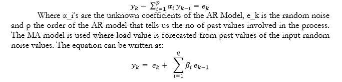
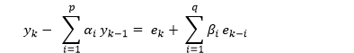
Where β_i’s  are the unknown coefficients of the Model, e_kis the random noise and q the order of the MA model. Written in the notation of ARMA (p, q), these models combine the strengths of the AR and MA model to forecast the load value. Present values of load can be expressed in the form of past values of load and current and past value of noise, as shown in the equation below:

[13] developed an ARMA model by adding Gaussian noise to incorporate nonlinearity and then selecting a suitable model, with an order, to predict load. Parameters are estimated using gradient-based methods, and finally, the model is validated for its adequacy with the real data. The model performed well compared to simple ARMA and ANN. [12] developed a basic ARMA model and compared it with Projection Pursuit Regression (PPR) to be better performing.

Another variant is Auto-Regressive Integrated Moving Average (ARIMA), which considers the non-linearity involved in a time series. The AR, MA, and ARMA models are applicable for stationary processes only. However, when non-stationary data is involved, data has to be transformed to a stationary form. The equation of the ARIMA model is:

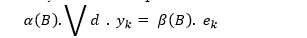
Where α, β are the unknown coefficients. e_k defines the noise. [14] an employed modified version of the ARIMA model by incorporating temperature and operator’s knowledge into the model.  The proposed model performed better than the ARMA model for predicting next year’s hourly data. The ARMA and ARIMA are used successfully by [11] to forecast the load for the Kuwaiti electric network. Their approach mainly uses segmentation and decomposition of time series into similar regions and contours to make the forecast.

Kalman Filtering Algorithm

A certain level of uncertainty generally terms long-term forecasting. To cope up with this, Kalman Filters were introduced in 1960 to minimize the mean of the squared model’s error. The algorithm comprises a set of equations that gives efficient recursive means to estimate the state of an observed sequence [15]. This technique has few powerful characteristics where it can control the highly noisy systems and cater to small unknown variables of the system. This algorithm can address unknown variables like weather, abrupt load demands, and customer requirements in load forecasting. The mechanism works in two stages. In the predictor stage, the algorithm predicts the load’s current state based upon its previous states. Its covariance and the corrector stage information from the metering device are collected to an estimated state vector by employing the weighted average. The Kalman Filter method generally does not take into account the non-linear issues of load forecasting. Hence its modified versions are employed as done by [15]. The proposed modified Kalman Filter versions Extended Kalman Filter (EKF) and Unscented Kalman Filters (UKF) to estimate the non-linear behavior better using Jacobian Matrices.

Regression Models

Regression models are widely used statistical methods in forecasting. The main gist is learning more about the relationship between dependent and independent variables of the process. Multiple regression is based on minimizing the sum of squares of the difference between observed and predicted values. [16] used regression technique to develop a semi-parametric additive model for 24-hour demand forecast. They developed 48 models on a half-hourly basis, using selected historical load and temperature data. Forecast residuals and forecast errors are calculated using the modified bootstrap method, and finally, empirical distributions are constructed around the forecast errors for load prediction.

Non-Linear Predictors

Non-linear dynamics of the power industry are explored using non-linear chaotic dynamic and evolutionary strategy by many studies. [17] used non-linear chaotic dynamic based predictor PREDICT2 for analysis of non-linear load during training stage with emphasis on optimizing the objective function. A new Evolutionary strategy is proposed to solve the optimization problem with a candidate solution vector, having a random value with a standard deviation. [18] applied Long Short-Term Memory (LSTM) and Gated Recurrent Unit (GRU) networks to remove gradient problems in the past load data for ELF.

Exponential Smoothing (ES)

This forecasting technique works on the weighted average of the past observations. The highest weight is given to the present value of the load, then the next lower weight to the preceding value of the present value and even lower to the observation before. Due to the simplicity and accuracy, the ES technique is used quite frequently for load forecasting. The ES techniques have been divided into three further divisions. Single exponential smoothing (Brown’s Method) is used when there is no pattern in the given data, Double exponential smoothing (Holt’s Method) when the trend is observed in the data, and finally, Triple Exponential Smoothing (Holt-Winters Method) when data reveals significant seasonal configurations. [19] Developed five ES weighted models, including a Singular Value Decomposition SVD based model to reduce the data to lower dimensions with uncorrelated variables. In [20], they proved that their proposed Seasonal Holt-Winters Exponential Smoothing method outperformed ARMA and PCA models. They used the models to forecast the seasonal demands of European data. They added an index and smoothing equation for forecasting the load. Also, ARMA and PCA models are developed to compare the performance. [21] Calculated load forecast for Irish market using Double Seasonal Holt Winter’s Exponential Smoothing with Error Correction. Seasonal parameters are initialized from the historical load data, and a model is proposed using the exponential smoothing algorithm. Finally, the GRG nonlinear error of predicted value and actual data is calculated. 

Artificial Intelligence (AI) Models

AI systems have been developed for forecasting and estimating with the advent of advanced technology and high computational powers.

Support Vector Machines (SVM)

Presented by Vapnik in 1995, the SVM is classification and regression techniques. SVM mainly extracts the decision rules having satisfactory generalization ability from the training data called support vectors [22]. Input space is mapped nonlinearly into a higher space dimension constructing an optimal hyper plane.  In the training phase of the SVM, linearly constrained quadratic programming is carried out, which is unique but time-consuming. [23] used Self Organizing Mapping (SOM) technique to organize the input data into clusters. SVMs are then applied to each data subset to forecast the load for the next day. This hybrid method proved helpful in addressing the non-stationary load time series. [22] and [24] applied VMD is applied to decompose input data into subseries based on the certain center frequency and bandwidth. The nonlinear mapping function is used to map data in a high dimension, where the SVR function is used to relate forecast values with input.

Artificial Neural Network (ANN)

Developed in 1990 by Warren McCulloch and Walter Pitts, the ANN has been applied in several areas, including forecasting and classifications [25]. ANN is a non-linear circuit that can perform non-linear curve fitting. It processes information in line with the human biological systems. Inspired by the working of the human brain, the NN can process a certain piece of information using its basic unit called a neuron. Information received at the input node of the neuron is accumulated, processed, and then further forwarded to the next neuron through the output node. The ANN system is trained on the relevant historical data to identify the similarities and patterns of the input data. Then based upon this prior knowledge about the data and system, the network gives generalized output. In its most simplistic form, the network consists of an input layer, a hidden layer, and an output layer.  The input I am sent to the hidden layer and associated weights performs a certain function f(x) to give an output. Based upon its topology, the ANN is generally categorized into Feed Forward (FF-NN) and Feedback or Recurrent NN.

Feed Forward Neural Networks (FF-NN)

Usually preferred for forecasting and consists of various combinations of input, hidden, and an output layer. In its simplistic form Single Layer Perceptron, no hidden layer exists. The forecasts are obtained using a linear combination of inputs and weight vectors, which are obtained using a learning algorithm that minimizes some cost function e-g MSE. With the addition of an intermediate layer, the NN takes Non-Linear Multi-Layer Perceptron (MLP). Neurons are arranged in layers and connected through weight vectors with the next layer. Neuron b takes the input from its predecessor neuron, if it exists, computes the weighted sum w, eliminates the bias, and gives the output after applying the activation function g. The equation is given by:

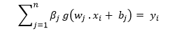
Where, x_i is the input, w_j is the weight, b is the neuron of hidden layers.

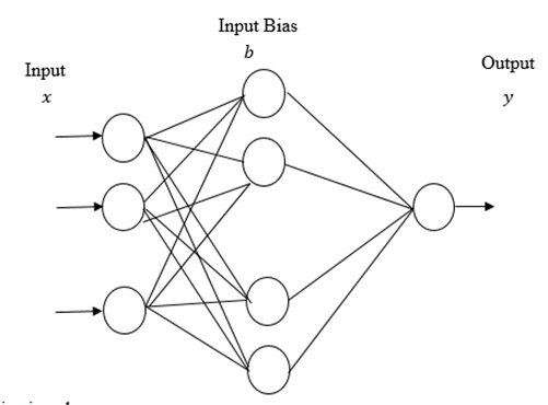
Figure 2. Basic Structure of a NN

Feedback Neural Networks           

Unlike the FF-NN, the feedback NN is dynamic. Whenever a new input pattern is given the output of neurons is computed. Their output depends on the state of the system. Feedback of the neurons is modified due to the feedback system, and hence the NN enters into a new state. To overcome the vanishing gradient problem of the NN, Nonlinear Autoregressive Models with Exogenous Inputs (NARX) have been developed. This three-layer FF-NN with good learning capabilities has a sigmoid activation function in its hidden layer, linear activation function in the output layer, and delay lines for storing previously predicted values.

NN-based STLF has been enhanced using Multi-resolution analysis (MRA) by [26]. Four models are developed with different input variables among load, temperature, differenced load from the first, and MRA with the differenced load. The final models comprise sub-models of the first three models to decompose the load series using individual fitting. The proposed Model with load, temperature and first-order differenced load as input predicted the load most accurately. [25] also proposed Wavelet-based NN (WNN), using previously used algorithms for generation, selection, and generalization, to compare its prediction performance. However, they concluded that results of WNN are comparable with naïve methods and MLP NN on GEFCom dataset. [27] improved the BP NN with the introduction of GA. They used PSO to improve the convergence speed and PCA to reduce the matrix dimensionality.

[28] introduced Artificial Immune System with ANN. The aim is to check the benefits of the robust AIS like computational strengths as its distributed, diverse, anomaly detection, and self-organizing learning abilities. The performance of AIS-based FF-NN has comparable results on the MAPE scale with that of BP NN. However, further studies may reveal the true potential of AIS in the field. Different types and scales of NN have been used for the last two decades by researchers for load forecasting. Having received considerable success, the NN is also criticized for having too many input parameters, leading to data overfitting. [29] conducted a detailed review of various models of NN with traditional statistical methods. They compared large NN with linear models, including Naïve forecasting, methods with one and more smoothing filters, smoothing filters with linear regression combination of smoothing filers, and NN. The conclusion is that large NN can perform well because they consider more historical data and can interpolate high dimensional functions, which improves the profile load forecasting. [30] also worked to investigate the non-linear characteristics of the power load series is identified using MLP. An attractor is then developed in a phase plane to train ANN. [31] proposed a set of probabilistic models as constrained quantile regression models to average and predict the future data.

While using NN [32] employed a wavelet-based ensemble scheme. Selection of mother wavelet and decomposition level is a tricky affair. Here ensemble of wavelets is used, and their output is aggregated to get the best features as output. Wavelet-based ensemble networks, algorithm incorporating Levenberg–Marquardt (LM) for improved learning, Conditional Mutual Information Feature Selection (CMIFS) method is employed for feature selection, and Partial Least Square Regression (PLSR) is used for forecasting purposes. In another scheme, [33] exploited that NN learns load dynamics without memorizing the data for a long time with accurate results. Challenges are faced while extrapolating the relationships different from those extracted from training data. Five models of three-layered FF NN are used for forecasting. Redundant hidden neurons are also eliminated by observing duplication in co-linearity with the output.

Hybrid Models

Many in the past have published applications of combining the strengths of different models into hybrid models. Also, for load forecasting, various methods have been combined to produce efficient methods. The probabilistic nature of power systems makes it a potential field for employing various methods to estimate the forecast for time.

Results

Since there is no gold standard yet for forecasting and methods for prediction, reviewers consider various assumptions while comparing the publications. This study assumes that all the results published in the studies are correct, methods used by the majority of the expert community are best. However, for statistical analysis, MAPE percentages of all studies are also compared.

Comparative Analysis

After selecting publications for this study during the initial phase, each publication has been studied in detail for comparative analysis as elaborated in Table III. The dynamics of the topic and unpredictability of load influence the researchers to use different variables and performance standards to measure their proposed methods. In addition, heterogeneity of data due to socio-economic conditions and consumer’s profile, non-linear environmental conditions, including weather, humidity for different countries, add complexity to the comparison of studies. At times a simple or a particular method favors a particular situation, even the sophisticated techniques. This study focuses on the comparison benchmarks mentioned in Table II, including Proposed Method, Data set used, Overview, and Prediction Term. ANN stands out to be the most used method for ELF after going through all the publications during this study, as shown in Graph II.

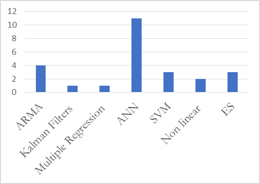
Graph 2.  No of Publications Studied as per Method

Eleven out of 25 publications has been used ANN in one form or the other. ARMA-based models are the next most frequently used method for ELF by the researchers.

Table 3. Comparison of Studies

Ref	Technique	Dataset/ Training & Testing	Overview
[12]	Hybrid using Auto-regression Integrated moving average (ARIMA) & projection pursuit regression (PPR)	5 min interval time series of Sichuan Electric Power Company, China with 864 observations for randomly selected data from 26-28 Sep 2016. 576 for training and 288 for testing out of the total of 864	·   ARIMA is modeled, estimating its order and parameters using Bayesian Information Criteria (BIC) and correlation function. ·   Next, the PPR model is developed. Integration of both models is carried out to address the linear and non-linear dynamics of the load forecast.
[11]	Hybrid model using Autoregressive Moving Average ARMA and ARIMA.	Daily load data of Kuwaiti Electric network from 2006 – 2008.	·   Data is segmented to locate the identical patterns and calculate their probability. Afterward, the series is decomposed using MA for load pattern segmentation. ·   For load forecasting, curve fitting is conducted to identify region similarity, contours, and related points.
[13]	ARMA including Gaussian and Non-Gaussian Processes	Hourly data of 3 months between 1998-1999 of Taipower Company, Taiwan	·   Historical data is processed for the Gaussian test using the Bi-spectrum process. ·   If data is Gaussian, second-order statistics are calculated; otherwise, the MA model is applied. ·   The correct model identified in the previous step is used to estimate the parameter representation of the model.
[14]	ARIMA Model integrated with operators knowledge	Hourly load and peak load data from Iran’s national grid from 1996-1998. Data from 1996-1997 is used for training, while that of 1998 for testing purposes.	·   ARIMA model is proposed considering the historical data, estimating the parameters. ·   16  Modified ARIMA models are used for forecasting along with the temperature and operators knowledge
[18]	Long Short-Term Memory (LSTM) and Gated Recurrent Unit (GRU) networks	Three-year record data of various feeders from West Canada with 1997 records 1,597 records for training and 400 out of total 1997 (80%/20% split ratio)	·   Features from past data are collected based on socio-economic and weather conditions. ·   Principal component analysis (PCA) and Normalization of selected features are performed. ·   LSTM and GRU networks for Many to Many and One to Many configurations are developed. ·   These networks are better to vanish and explode gradient problems in the data.
[17]	A hybrid approach based on non-linear chaotic dynamic predictor	Hourly electricity load of the year 2002 from New England, Albert, and Spain. Random selection of 4 weeks, one each in 4 months of a year, for testing. Rest of the data used for training	·   The time-series data, set as input to the model, is divided into two segments. One segment is used to predict data in the second segment. ·   The population is initialized using candidate random variables. Next, the population parameters are recombined to produce off-springs and then mutate. ·   This ES is used to tune the prediction parameters.
[16]	Semiparametric additive models using Modified Bootstrap method	Half hourly demand and temperature data of Melbourne from 1997-2009 from Australian National Electricity Market. Data from 2004-2008 was used for training, and 2009 data for testing.	·   A Semiparametric model is developed to forecast demand and temperature values using their historical data. Cross-validation is done to select the variables for use in models. ·   Forecast residuals are calculated by sequentially substituting into random forecasted model values. ·   The modified bootstrap method is used to obtain forecast errors.
[15]	Modified Non-linear Kalman Filter, Extended Kalman Filter (EKF), and Unscented Kalman Filter (UKF). Weather and Wind Speed data is accumulated from the website.	Reference Energy Disaggregation Dataset (REDD) anonymously collected from Boston, US	·   Standard KF is modeled using past data, temperature, and wind speed data. ·   The model predicts the value based on past data along with its covariance. ·   The output is recursively updated using the law of minimizing mean square error. ·   The non-linear Modified filters, EKF and UKF, are applied to calculate the prediction.
[12]	ES with Holt-Winters, ARIMA, and PCA	30 Weeks hourly/ half hourly data of 6/ 4 European countries from Apr-Oct 2005. The first 20 weeks of each data is used for training and the last ten weeks for testing.	·   Seasonal Holt-Winters Exponential Smoothing is applied to forecast two seasonal demands. ·   Additional seasonal index and extra smoothing equations are added for the double seasonal method. ·   The initial level and seasonal values are estimated by averaging the observations and minimizing the squared sum of errors. ·   ARMA and PCA models are also developed to compare the performance
[21]	Double Seasonal Holt-Winters Exponential Smoothing with error correction	Half-hourly data of 15 months from an Irish supply company from Jan 2013- March 2014	The seasonal parameters defined in Days, Weeks, and Seasons are initialized from the historical load data. The model is proposed using the exponential smoothing algorithm. Finally, the GRG nonlinear error of predicted value and actual data is calculated.
[19]	Five exponentially weighted methods incl new Singular Value Decomposition SVD based ES	Half hourly observation from 2007-2009, first two years used for training and last year for testing	·   SVD based approach is used to reduce the data to lower dimensions with uncorrelated variables. ·   Modified Holt Winter ES (HWT) ·   Discounted weight regression (DWR)
[23]	A hybrid approach to combine SOM with SVM	Hourly data of one year from 2003-2004 of New York City, US	·   In the first stage, SOM is used to group the training data with similar properties. ·   The SVM network of 24 machines is then applied with regression and risk minimization principles to forecast the next day’s load.
[24]	Simulated Annealing with SVM	Taiwanese load data from 1045-2003, 40 years training set from 1945-1984, 10 yrs validation 1985-1994, 9 yrs testing 1995-2003	·   The past data is normalized using the simulated annealing algorithms. ·   Then SVMs are applied for load forecasting. ·   The proposed model is compared with ARIMA and Regression NN.
[22]	Hybrid model using Variational Mode Decomposition Self Recurrent Support Vector Regression Cuckoo Bird Cuckoo Search (VMD-SR-SVRCBCS)	Half-hour load data from National Electricity Market, Queensland, Australia, and hourly load data from New York Independent System, USA. Both datasets were distributed into 3 x parts for the training, validation, and testing phase	·   VMD is applied to decompose input data into subseries based on certain center frequencies and bandwidth. ·   The nonlinear mapping function is used to map data in a high dimension, where the SVR function is used to relate forecast values with input.
[30]	ANN-based on Multilayer Perceptron	Daily peak demand of one year for 1995, 9 months data is used for training and two months for testing	·   The time series is extended to confirm its chaotic character using correlation dimension and Lyapunov Spectrum. ·   The state-space of a differential equation is created for the time series taking into account all its variables. ·   Then model based on correlation dimension and state space of the data is developed.
[27]	Neural Network optimized using Particle Swarm Optimization (PSO) and Principal component analysis (PCA)	1-year data of a Power Grid Corporation Previous one-year data for training	·   PSO is used to initiate the model from initial weights and thresholds. ·   PCA is used to reduce the input dimension as per the set threshold with GA optimization. ·   Load is forecasted for the next 24 hours.
[28]	Feed Forward-Neural Network (FF-NN) trained by the Artificial Immune System (AIS)	Day, time, temperature, and 720 samples each from historical load data of Kuala Lumpur, Malaysia, and the other from North Carolina, US 65% of the data is used for training and 35% for testing	·   The AIS-based algorithm is developed with initial weights selected randomly between 0 and 1. ·   FF-NN on MLP architecture is proposed where input parameters are multiplied with weights. ·   Regression is performed to correlate the predicted values with the past load series.
[34]	Convolutional Neural Network (CNN) with K Means clustering is employed.	1.4 million records of electricity data from 2012-2014 containing hourly load data from the power industry. 1,003,716 samples from 2012 - 2013 are used for training and 469300 samples for testing.	·   Raw data is pre-processed, converted into two subsets, training and testing, based upon selected feature analysis using K Means Clustering. ·   CNN is trained on one subset and then validated on the testing subset.
[35]	Feed Forward Deep Neural Network (FF-DNN) and Recurrent Deep Neural Network (R-DNN)	Hourly data of NEW England, the USA from 2007-2012 comprising 52600 records. 43824 samples are used for training, while the rest are used for the testing phase.	·   The data is analyzed in the time and frequency domain to model it comprehensively. ·   In the next stage, Rectifier Activation Function (ReLU) is used to model FF-DNN and R-DNN. ·   Separate results are computed considering only Time Domain and Time & Frequency Domain features.
[36]	Modified Deep Residual Network adopting ensemble strategy	North American utility data set with hourly data from 1985-1992. 2-year data from 1991-1992 is used as test data, rest of the data is used for training. To check the generalization, ISO-NE data is used.	·   A two-level basic structure is formed for forecasting 24 hours data with the Scaled Exponential Linear Units (SELU) activation function. ·   Output is fed into Deep Residual Network (ResNet) constructed from a stack of three residual blocks. ·   Modifications are made, ResNetPlus, by employing several residual side blocks and averaging the output of each main residual block with these side blocks to improve error backpropagation of the network. ·   The next ensemble strategy is used to improve the generalization capability of the network.
[26]	NN with Wavelet decomposition	Hourly load data of North America from 1988-1992	·   Features are extracted into Low and High-Frequency components using Multi-Resolution Analysis. Input variables are selected by applying correlation functions. ·   Four models of NN have been developed based upon MLP. ·   The model with inputs of load, temperature, and first-order differenced performed the best among other NN.
[37]	Wavelet Neural Networks	Hourly load data of NEW England from 2003-2005 as training and year 2006 data used for testing.	·   Wavelets are used to decompose the load into Low and High-Frequency components ·   MLP based NN is then applied for load forecasting.
[29]	Large NN and regression methods	Hourly data from 1996-1997 of a city of Brazil. Data is split for the training, testing, and validating phase.	·   Various models are developed based upon Naïve forecasting, methods with one and more smoothing filters, smoothing filters with linear regression combination of smoothing filers and NN and large NN
[33]	NN	Load data of the previous 1 hour is used to predict the next 20 minutes load for a power company in the US.	·   They used relative load curves of past data instead of load increments to improve the forecasting accuracy as is done in traditional NN models. ·   Input variables are selected based upon their string statistical correlation with outputs. ·   Supervised training is carried out for the proposed NN using the previous load data and minimizing the error function.
[38]	Hybrid NN based on Wavelets	Hourly load data from ISO England for the year 2009-2010.	·   ELM-LM algorithm is developed by randomly initializing the weights and biases to estimate the output weights. ·   Wavelet transform is used to employ frequency components along with temporal dimensions of the past load series. ·   PLSR is used to combine the forecasts of different wavelets. ·   Hourly load data is fed into 24 FF-NN with the detailed extraction of frequency components using wavelet transforms.

Statistical Analysis

For performance measurement, researchers have used various forecasting standards like including Mean Absolute Percentage Error (MAPE), Root Mean Square Error, etc. However, MAPE is used more frequently in statistical studies. The difference value was calculated by taking the absolute difference between the proposed method and other methods with which it is compared.  The MAPE difference of the proposed and other methods were calculated. Then the smallest value is located to identify the best method as depicted in Table 4. It is revealed that ARMA models and ANN gave the lowest MAPE values. A stable difference criteria has also been defined by setting the value of alpha from 0.01 to 5. This means that difference values less than 0.01 and greater than 5 were ignored in this study. The mean MAPE for ANN and ARMA Models is 0.799 and 0.8446, respectively.

Table 4. Comparison of MAPE and Standard Deviation.

Cat	Ref	Proposed Method	Benchmark Method	% MAPE	Mean-MAPE
ARMA / ARIMA	[12]	Hybrid using ARIMA & Projection Pursuit Regression (PPR)	ARIMA PPR	0.634 0.403	0.8446
	[11]	Hybrid model using ARMA and ARIMA.	Real data	0.5
	[13]	ARMA including Gaussian and Non Gaussian Processes	ARMA ANN	0.05 0.58
	[14]	ARIMA Model integrated with operators knowledge	ARIMA ANN Operators	1.24 1.27 2.08
Non-Linear	[18]	Long Short-Term Memory (LSTM) and Gated Recurrent Unit (GRU) networks	FNN Modified FNN	5.1 2.79	5.05
	[17]	A hybrid approach based on non-linear chaotic dynamic predictor	ANN ARIMA	5 4.5
Regression	[16]	Semi parametric additive models using Modified Bootstrap method - Regression	ANN Hybrid	0.85 0.4	0.85
Kalman Filter	[15]	Modified Non-linear Kalman Filter - Kalman	EKF	0	0
Exponential Smoothing (ES)	[20]	ES with Holt Winters.	ARMA PCA AR	0.059 0.05  0.086	0.69
	[21]	Double Seasonal Holt-Winters Exponential Smoothing with error correction	Naïve w/o EC	1.66 5.3
	[19]	Five exponentially weighted methods incl new Singular Value Decomposition SVD based ES	ANN HWT with SM NEW SVD Weather-based	0.02 0.01 0.01 0.016
Vector Machines (SVM)	[23]	Hybrid approach to combine SOM with SVM	ISO SVM	1.15 0.65	2.42
	[24]	Simulated Annealing with SVM	ARIMA GRNN	8.55 3.42
	[22]	Hybrid model using VMD-SR-SVRCBCS	ARIMA GRNN BPNN SVR	7 5.3 5.1 3.8
Neural Networks (NN)	[30]	ANN based on Multilayer Perceptron	Others	0.4%	0.799
	[27]	NN optimized using PSO and PC Analysis	No PC Reduction	1.1
	[28]	FF-NNtrained by theArtificial Immune System (AIS)	Data 1 - AIS Data 2 – AIS	0.473 1.347
	[34]	CNN with K Means clustering is employed.	LR SVR SVR &K Means NN NN & K-Means	25 8.97 0.89 0.163 0.115
	[35]	FF-DNN and Recurrent Deep Neural Network (R-DNN)	Time Frequency	12 0.01
	[36]	Modified Deep Residual Network adopting Ensemble Strategy	Temperature-1 Temperature-2 Temperature-3	0.02 0.05 0.11
	[26]	4 models based on NN with Wavelet decomposition with different inputs	Model-1 Model-2 Model-3	0.17 0.42 0.94
	[37]	Wavelet NN	NN w/o weather NN & weather Similar day	0.188 0.07 0.22
	[29]	Large NN and regression methods	Smoothing with small NN  Large NN	0.1 1
	[33]	NN	Forecaster-1 Forecaster-2 Forecaster-3	0.59 0.39 0.23
	[38]	Hybrid NN based on Wavelets	Abductive MLR RBFNN Random forest	0.79 0.83 0.56 0.92

Discussion and Future Research.

Load forecasting has become a topic of significance in the past few decades. Researchers have used various techniques to identify the best-performing methods. However, the non-linear dynamics of the topic imply that no one method can be classified as the best. Availability of historical load data is the prime factor in forecasting. However, heterogeneity in this data itself challenges the analysis. The data was dispersed in different patterns with different power companies. It was calculated on an hourly basis, whereas at the other places, it is recorded on a seasonal basis.

Most of the statistical methods employ past load series and weather information for prediction. These past load data were used as input to Regression techniques and the weather and its functional relationship. The same was then solved regressively to reduce the square error of the prediction. Exponential smoothing models were developed by a linear combination of time series and other variables. Kalman filtering used filtering techniques to reduce the noise in data to predict future load. When combined with Wavelet decomposition forecasting was improved further as it employed frequency component of data series as well. The ANN techniques have been performed quite well for ELF. However, their main concern was data fitment. The NN employed layers of neurons and a large number of parameters that raised the concern over parameterization in performing the task. Large NN performs better in forecasting results, but the theory behind this remains a black box.

Meteorological conditions also risk load forecasting. Although in today’s digital world, previous data and future weather forecasts are also available. Still, the unpredictability of the weather, humidity conditions plays a significant role in load forecasting. Then the socio-economic conditions of the consumers dictate the variability of load demands. One cannot consider the functions, gatherings, or other related activities at a specific place. Another important concern is about the transmission network dynamics. Equipment failures and accidents make the power unavailable in one region, thus causing demand at another generating region.

Technological advancements, especially in the form of renewable energies, have modified the dynamics of power sectors. The load forecasting will be an area of concern to fulfill consumer’s power requirements. Based on this study, the following areas are elaborated for future research:

• Implement the techniques found during this study on the real-world load data to verify their performance. Challenges found in this study, like availability of data, weather constraints, diverse consumer power demand, etc., will be considered.
• Increasing use of electric appliances and wide adoption of electrical transportation systems significantly impact electricity requirements. Load forecasting in this regard will enable power utilities to meet user’s load requirements.
• Load forecasting is evolving day by day with the latest technological developments. The growing acceptance of renewable power generation systems, especially solar systems, makes users' load demand unpredictable. Research in renewable power generation and forecasting is also an area of interest for the future.
• Study the feasibility of integrating renewable power generation systems into the main power grid.

Conclusion.

Meta-Analysis is carried out by studying 25 publications on ELF modeling proposed by researchers and compared with various other forecasting methods. The criterion for comparison is selected, including technique employed, data set used, overall methodology, performance, and MAPE measurement. The comparative results show that various non-linear factors play a significant role in ELF, importantly weather conditions. Few methods are preferred because of their fast computation power and linear relationship among variables. ANN and ARMA are found to be the best performing methods. ANN is mostly used when changes occur at a faster pace like frequent changes in weather or environmental conditions. However, with larger NN, the issues of data over fitment need to be taken into consideration. The ARMA models are attractive due to ease in their practical interpretation. They are usually criticized for their limitation to deal with non-linearity behavior of processes.

Author’s Contribution. All the authors contributed equally.

Conflict of interest. We declare no conflict of interest for publishing this manuscript in IJIST.

Project details. Nil

References:

1. Hammad, M. A., Jereb, B., Rosi, B., & Dragan, D.. Methods and Models for Electric Load Forecasting: A Comprehensive Review. Logistics & Sustainable Transport, (2020)11(1), 51-76.
2. Weron, R.. Electricity price forecasting: A review of the state-of-the-art with a look into the future. International journal of forecasting, (2014), 30(4), 1030-1081.
3. Leung, T. C., Ping, K. P., & Tsui, K. K. What can deregulators deregulate? The case of electricity. Journal of Regulatory Economics, (2019),56(1), 1-32.
4. Kuster, C., Rezgui, Y., & Mourshed, M.. Electrical load forecasting models: A critical systematic review. Sustainable cities and society, (2017),35, 257-270.
5. Zhao, H., & Tang, Z. The review of demand side management and load forecasting in smart grid. In 2016 12th World Congress on Intelligent Control and Automation (WCICA) 2016, (pp. 625-629). IEEE.
6. Zor, K., Timur, O., & Teke, A. A state-of-the-art review of artificial intelligence techniques for short-term electric load forecasting. In 2017 6th International Youth Conference on Energy (IYCE) (pp. 1-7). 2017, IEEE.
7. Almalaq, A., & Edwards, G. A review of deep learning methods applied on load forecasting. In 2017 16th IEEE international conference on machine learning and applications (ICMLA), 2017, (pp. 511-516). IEEE.
8. Upadhaya, D., Thakur, R., & Singh, N. K. A systematic review on the methods of short term load forecasting. In 2019 2nd International Conference on Power Energy, Environment and Intelligent Control (PEEIC). pp. 6-11, 2019. IEEE.
9. Mohammed, Z. C., Humberto, A. R. J., Kiplel., M. C. & Chepkoech, M. A Meta-Analysis on Sustainable Supply Chain Management: An Analytical approach. European Journal of Logistics, Purchasing and Supply Chain Management, 2017.
10. Neuman, L. W. (2007). Social research methods, 7/E. Pearson Education India.
11. Almeshaiei, E., &Soltan, H. A methodology for electric power load forecasting. Alexandria Engineering Journal, 2011, 50(2), 137-144.
12. Yang, L., & Yang, H. A Combined ARIMA-PPR Model for Short-Term Load Forecasting. In 2019 IEEE Innovative Smart Grid Technologies-Asia (ISGT Asia) (pp. 3363-3367). 2019. IEEE.
13. Huang, S. J., & Shih, K. R. Short-term load forecasting via ARMA model identification including non-Gaussian process considerations.IEEE Transactions on power systems, 2003, 18(2), 673-679.
14. Amjady, N. Short-term hourly load forecasti using time-series modeling with peak load estimation capability.IEEE Transactions on power systems, 2001, 16(3), 498 505.
15. Gaur, M., &Majumdar, A. (2017). One-Day-Ahead Load Forecasting using nonlinear Kalman filtering algorithms.
16. Fan, S., & Hyndman, R. J. Short-term load forecasting based on a semi-parametric additive model. IEEE Transactions on Power Systems, 2011, 27(1), 134-141.
17. Unsihuay-Vila, C., De Souza, A. Z., Marangon-Lima, J. W., & Balestrassi, P. P. Electricity demand and spot price forecasting using evolutionary computation combined with chaotic nonlinear dynamic model. International journal of electrical power & energy systems, 2010, 32(2), 108-116.
18. Dong, M., & Grumbach, L. (2019). A Hybrid Distribution Feeder Long-Term Load Forecasting Method Based on Sequence Prediction. IEEE Transactions on Smart Grid, 11(1), 470-482.
19. Taylor, J. W. (2011). Short-term load forecasting with exponentially weighted methods. IEEE Transactions on Power Systems, 27(1), 458-464.
20. Taylor, J. W., & McSharry, P. E. (2007). Short-term load forecasting methods: An evaluation based on european data. IEEE Transactions on Power Systems, 22(4), 2213-2219.
21. Kavanagh, K. (2017). Short Term Demand Forecasting for the Integrated Electricity Market. Student Journal of Energy Research, 2(1), 1.
22. Zhang, Z., Hong, W. C., & Li, J. (2020). Electric load forecasting by hybrid self-recurrent support vector regression model with variational mode decomposition and improved cuckoo search algorithm. IEEE Access, 8, 14642-14658.
23. Fan, S., & Chen, L. (2006). Short-term load forecasting based on an adaptive hybrid method. IEEE Transactions on Power Systems, 21(1), 392-401.
24. Pai, P. F., & Hong, W. C. (2005). Support vector machines with simulated annealing algorithms in electricity load forecasting. Energy Conversion and Management, 46(17), 2669-2688.
25. Ribeiro, G. T., Mariani, V. C., & dos Santos Coelho, L. (2019). Enhanced ensemble structures using wavelet neural networks applied to short-term load forecasting. Engineering Applications of Artificial Intelligence, 82, 272-281.
26. Reis, A. R., & Da Silva, A. A. (2005). Feature extraction via multiresolution analysis for short term load forecasting. IEEE Transactions on power systems,20(1), 189-198.
27. Lv, Y. C., Xu, X., Xu, R. L., &Ren, H. (2019, January). Research on Short-Term Load Forecasting Approach for Smart Grid. In 2019 International Conference on Intelligent Transportation, Big Data & Smart City (ICITBS) (pp. 602-605). IEEE.
28. Hamid, M. A., & Rahman, T. A. (2010, March). Short term load forecasting using an artificial neural network trained by artificial immune system learning algorithm. In 2010 12th International Conference on Computer Modelling and Simulation (pp. 408-413). IEEE.
29. Hippert, H. S., Bunn, D. W., & Souza, R. C. (2005). Large neural networks for electricity load forecasting: Are they overfitted?.International Journal of forecasting, 21(3), 425-434.
30. Michanos, S. P., Tsakoumis, A. C., Fessas, P., Vladov, S. S., &Mladenov, V. M. (2003, July). Short-term load forecasting using a chaotic time series. In Signals, Circuits and Systems, 2003. SCS 2003. International Symposium on (Vol. 2, pp. 437-440). IEEE.
31. Wang, Y., Zhang, N., Tan, Y., Hong, T., Kirschen, D. S., & Kang, C. (2018). Combining probabilistic load forecasts. IEEE Transactions on Smart Grid, 10(4), 3664-3674.
32. Li, S., Wang, P., & Goel, L. (2015). A novel wavelet-based ensemble method for short-term load forecasting with hybrid neural networks and feature selection. IEEE Transactions on power systems, 31(3), 1788-1798.
33. Charytoniuk, W., & Chen, M. S. (2000). Very short-term load forecasting using artificial neural networks.IEEE transactions on Power Systems, 15(1), 263-268.
34. Dong, X., Qian, L., & Huang, L. (2017, February). Short-term load forecasting in smart grid: A combined CNN and K-means clustering approach. In 2017 IEEE International Conference on Big Data and Smart Computing (BigComp) (pp. 119-125). IEEE.
35. Din, G. M. U., &Marnerides, A. K. (2017, January). Short term power load forecasting using deep neural networks. In 2017 International Conference on Computing, Networking and Communications (ICNC) (pp. 594-598). IEEE.
36. Chen, K., Chen, K., Wang, Q., He, Z., Hu, J., & He, J. (2018). Short-term load forecasting with deep residual networks.IEEE Transactions on Smart Grid, 10(4), 3943-3952.
37. Chen, Y., Luh, P. B., & Rourke, S. J. (2008, June). Short-term load forecasting: Similar day based wavelet neural networks. In 2008 7th World Congress on Intelligent Control and Automation (pp. 3353-3358). IEEE.
38. Li, S., Wang, P., & Goel, L. (2015). A novel wavelet-based ensemble method for short-term load forecasting with hybrid neural networks and feature selection. IEEE Transactions on power systems, 31(3),1788.1798.