
Flow Analysis of Various Inlet Velocity Profiles on Indoor Temperature for Energy Conservation of HVAC System Using CFD
Atta ul Mannan Hashmi1, Arshan Ahmed1, Fahad Rafi Butt2, Shahbaz Ghani1 and Imran Akhtar PhD1.
1Department of Mechanical Engineering, NUST College of Electrical and Mechanical Engineering, National University of Sciences and Technology, Islamabad, Pakistan.
2Research Associate, Digital Pakistan Lab, NUST College of Electrical and Mechanical Engineering, National University of Sciences and Technology, Islamabad, Pakistan.
* Correspondence: Atta ul Mannan Hashmi; atta44009@gmail.com.
Citation | Hashmi. A. M, Ahmad. A, Butt. F. R, Ghani. S and Akhtar. I, “Flow Analysis of Various Inlet Velocity Profiles On Indoor Temperature For Energy Conservation of HVAC System Using CFD”. International Journal of Innovations in Science and Technology, Vol 3, issue, pp: 187- 196, 2021.
Received | Dec 14, 2021; Revised | Jan 25, 2022 Accepted | Jan 28, 2022; Published | Feb 06, 2022.
__________________________________________________________________________
Abstract.
Energy conservation has been the most popular topic of the modern world. Heating, Ventilation and Air Conditioning (HVAC) systems consume approximately 10 % of the total energy of world. In order to improve the efficiency of HVAC systems, two dimensional (2D) room with inlet, outlet and heat source has been modeled. ANSYS Fluent has been used for numerical analysis of air flow in a 2D room. User Defined Functions (UDFs), which are coded in C language and hooked in ANSYS fluent, have been used for recording temperature variations and for heat generation within 2D room. Besides studying velocity fields and temperature distributions within indoor environment under specified boundary conditions, reference region for comparative analysis is also selected during Steady State (SS) numerical simulations. During transient analysis, temperature variations of a selected location are recorded for four different scenarios under varying inlet velocity profiles i.e. three for 0°, 30°, 60° angle with 1.3661 m/s velocity and fourth 0° with 2.7322 m/s velocity. Temperature profile of reference region after 1500 sec of transient simulations are compared with the steady state. Temperature profile of the scenario once the air is injected at 30° closely matched with the steady state temperature profile of the selected region. Time for attainment of SS temperature is also measured and compared after transient simulations. SS temperature value was attained twice, first at 240 seconds when the air was injected at 0° with 2.7322 m/s and secondly at 522 seconds when inlet air entered at velocity of 1.3361 m/s at 30°. The power consumption by increasing the fan speed is much higher as compared to the power consumed for changing direction only.
Keywords: HVAC systems; energy conservation; computational fluid dynamics; user defined functions and heat generation.
Introduction
Study of indoor environment is relatively complicated owing to its dependence on velocity fields, temperature distribution and relative humidity maps. Study of indoor environment gets more complex once it comes to the presence of heat source within closed environment. HVAC systems are used in closed room for providing comfortable environment to the occupants. The fundamental phenomenon of convection governs the heat transfer within closed environment and keeps the temperature within comfortable zone. In the presence of heat source both natural and forced convections contributes towards heat transfer. Convection is a process of transferring heat from hotter to cooler medium by mass motion of fluids. In natural or free convection, hot air moves up and away from the hotter surface whereas in forced convection air is forced over the hot object for taking away heat and lowering its overall temperature. Heat transfer coefficient ‘h’ depends upon direction, magnitude of fluid flow and the temperature difference between the flowing fluid and the hotter object [1].
Over many years, various studies and analysis have been carried out to ascertain the air flow patterns and temperature gradient profiles within various geometrical boundaries. Major focus of the researchers have remained on forced convection rather than natural convection because heat transfer through the latter is considered negligible as compared to former. In 2D model, temperature distribution and velocity profile for free, forced and mixed convection with appropriate geometries and mesh refinement was presented by Horikiri et al. [2]. Although the CFD study was validated with experimental data for 2D empty room. But natural and mixed convections were achieved by keeping constant temperature boundary conditions only. Ni & Bai [3] presented the statistical research on air conditioning energy performances in data centers. HVAC systems constitute almost 38% of total energy consumed by data centers. Study also emphasized on the comfortable and optimum operating temperature range of 18°C~27°C which is also recommended by American Society of Heating, Refrigerating and Air-Conditioning Engineers (ASHRAE). Fang et al. [4] carried out Computational Fluid Dynamics (CFD) simulations in order to study temperature distribution of the air conditioned room both under steady and transient conditions. However, fixed inlet conditions and profiles were used for the analysis. Mesenhöller et al. [5] presented the effect of ventilation on the interior temperature distribution. Unsteady ventilation led to stronger mixing effects in the interior zone as compared to fixed and steady ventilation. Raczkowski et al. [6] validated CFD model with the experimental data for ensuring thermal comfort in a naturally ventilated rooms. Schiavon & Melikov [7] calculated the energy conservation of HVAC systems under different velocity inlet profiles. Wang & Chen [8] studied various turbulence models for the assessment of transitional flows within closed environment. The complexity of the experiment and simulation was gradually increased from isothermal forced convection in totally empty room to a room with box and then to a heated box.
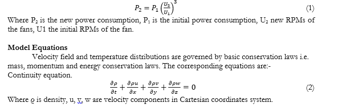
Study of the literature reveals that for economizing the energy consumption by HVAC systems, air distribution and temperature contours in closed environment under various circumstances plays the most pivotal role. Modeling and controlling HVAC system’s response under different conditions mainly depends upon the thermal comfort which includes, velocity field, temperature profile and relative humidity maps.
According to third fan law, just by doubling the initial velocity will result in 8 time’s increase of power consumption by the fan only. Third law of the fan is stated below:

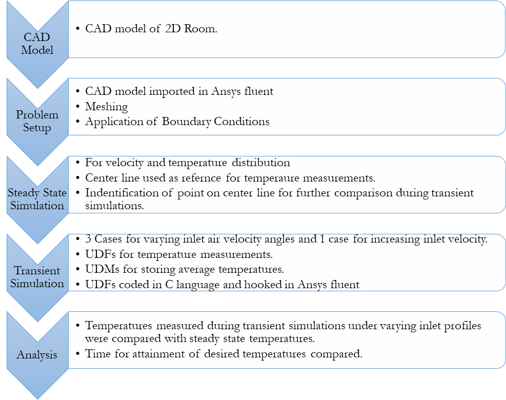
Methodology
Methodology adopted for numerical simulation is depicted in the following flow diagram:
Numerical Simulation
Geometry and Setup. A 3D cubic room [8] as depicted in Figure 1 has been used for analyzing velocity field and temperature distribution. In order to study the flow separation, a cubic box of half the dimensions of the room (1.22 x 1.22 x 1.22m) was used at the center. Cubic box was heated to study the effect of natural convection in a room. About 0.03m inlet and 0.08m outlet cross configurations were used for analysis.
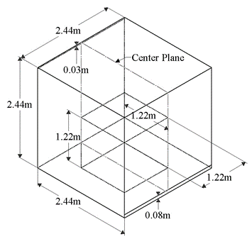
Figure 1. 3D CAD Model of Room under Consideration.
For the present study, center plane having inlet at top left and outlet at right bottom as shown in Figure 2.
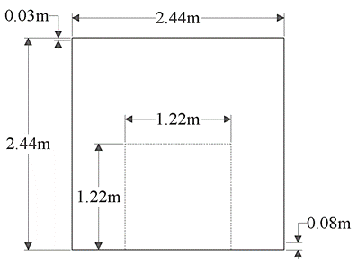
Figure 2. 2D CAD Drawing.
ANSYS fluent was used for numerical analysis. Complete 2D center plane of the room was discredited into 187,617 all quad cells of max size 0.005m. Inflation with first layer thickness of 0.0042m and growth rate of 1.05 was applied on all the edges with 5 layers as shown in Figure 3. k-ϵ Realizable with standard wall function turbulence model has been used for modeling turbulence. Semi Implicit Method for Pressure Linked Equations (SIMPLE) with second order upwind schemes have been set for pressure, momentum and energy whereas first order implicit scheme has been used in this analysis.
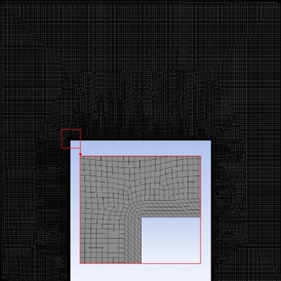
Figure 3.Mesh with Inflation at the edges.
Air was injected at 1.3661m/s with the constant temperature of 295.35K because same boundary conditions were used by reference [8]. A constant heat of 470.3W/m3 was generated from the box to simulate actual scenario and to cater for buoyant forces effect. Outlet boundary condition of pressure-outlet with zero Pascal of gauge pressure at 323.15K was set at the 2D room oulet. Initial interior temperature of the complete room was set at 323.15K.
For numerical analysis, case was initially run for steady state in Ansys fluent for obtaining velocity field and temperature distribution profile in the room. Center line as shown in Figure 6 was used as a reference for temperature measurements. For transient analysis, User Defined Function (UDF) of heat source was used for heat generation by the box and UDF (Execute at the END) was used to calculate average temperature around the center line as identified during steady state analysis. Both direction and magnitude of inlet air velocity profiles were varied in transient analysis depending upon already calculated average temperature of any identified point or region during steady state study. Present study only discusses the effect of change in direction and magnitude of inlet velocity at a constant temperature of 295.35K. Total of 4 cases excluding steady state were analyzed, out of which 3 cases for constant inlet velocity at clockwise 0°, 30° and 60° with the top wall. Last case was analyzed with the doubled velocity at 0° and constant temperature of 295.35K.
Validation and Verification.
Air distribution in a cubic room with the heated box was validated for constant inlet velocity of 1.3661 m/s and isothermal boundary conditions. Figure 4 depicts the heat generation by the box within a cubic room.
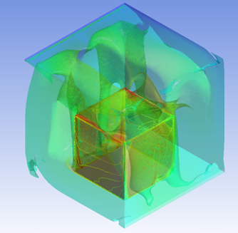
Figure 4. Temperature Iso-Surfaces inside a Cubic Room with Heat Generation.
The results from the current simulations are compared with Wang & Chen [8] for validation before carrying out further analysis. The comparison plot of normalized x-velocity with the normalized height is validated in the Figure 5.

Figure 5. A Comparison of Present Simulation with the Experimental Data.
Results
In order to simplify the analysis, center line was selected and its variations were studied with changing inlet profile. A point (1.22, 1.503) on the center line was chosen which had the maximum gradient below which the effect of heat generation source takes over. The steady state temperature contours along with the chosen point and velocity magnitude contours are shown in Figure 6&7 respectively.
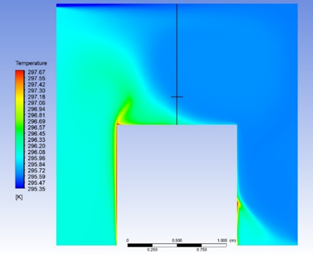
Figure 6. Steady State Temperature Profile.
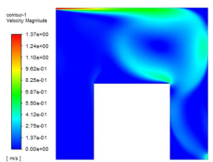
Figure 7.Steady State Velocity Magnitude Contours.
Temperature was measured at the center of each cell of the selected rectangular region around centerline as depicted in Figure 8. Average temperature of the region was calculated at the end of each iteration during steady state and after every time step during transient analysis. UDFs were separately coded and hooked in ANSYS fluent for recording live data during the simulation. Average temperature was stored separately in a User Defined Memory (UDM) for analysis purpose. Calculated average temperature can be used for continuously changing inlet velocity or temperature profiles. For simplicity and focusing on direct effect of inlet profiles on temperature distributions, UDF was only used for calculating average temperatures under different fixed inlet velocity profiles represented in Figure 8.
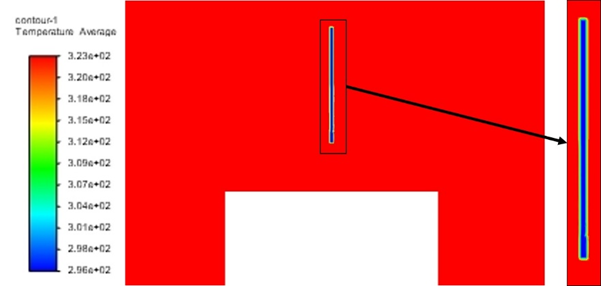
Figure 8 UDM Temperature Contours.
Transient Analysis. Transient analysis was run for 1500 seconds of physical time for three cases with constant velocity inlet (1.3661 m/s) at 0°, 30° and 60° of flow angles clockwise with the top wall. The transient response for the center line differed from the steady state response. The variation in the temperature profiles of center line during steady state and transient simulations (after 1500 seconds of physical time) are shown in Figure 9.
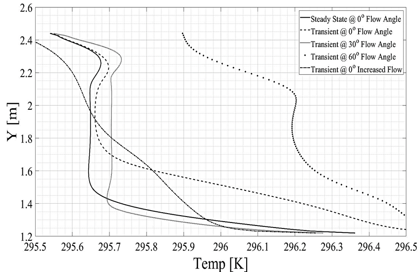
Figure 9.Center Line Temperature Variation Plots.
Solid line in the graph (Figure 9) represents steady state variations. Dashed, dotted and dashed-dot lines shows constant inlet velocities at 0°, 30°, 60° clockwise angles with the top walls whereas ‘o’ plot shows the velocity variations with doubled inlet velocity i.e. 2.7322 m/s. Center line graphs showed that overall profile of inlet velocity injected at 30°, matches with the steady state profile with further decrease in temperature below 1.428m of height. Although overall profile of flow injection at 30° was shifted towards right by 0.05K but the overall temperatures values below the height of 1.428m were lower than the steady state injection at 0°. The overall center line of height (1.5 ~2.16m) averaged temperatures of all the four cases along with the steady state bench mark as shown in Figure 10. The averaged center line temperature at 30° is 0.11K less than the inlet at 0° at same constant velocity.
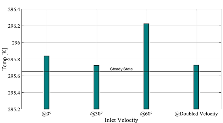
Figure 10. Center Line Averaged Temperatures.
Area averaged temperature of the complete room was also calculated for 1500 sec of transient simulation. Comparative analysis as shown in Figure 11 revealed that the overall averaged room temperature at 30° is 0.0273K less than the velocity inlet at 0°. Averaged area room temperature for doubled velocity (2.7322 m/s) inlet at 0°is 0.3044K less than velocity (1.3661 m/s) at 0°.
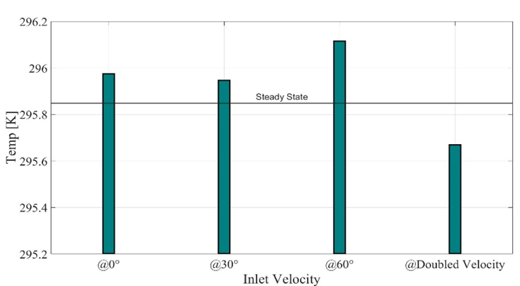
Figure 11.Area Averaged Temperatures of Room.
The minimum temperatures achieved at the selected point (1.22, 1.5) was also compared for better analysis. Although with the change in selection (point or region), the values of temperature may produce results much different from the one shown in Figure 12. But overall averaged room temperature and the time it takes to reach will contribute towards energy conservation.

Figure 12. Min Temperatures of a Point (1.22,1.503).
Discussion
After 1500 seconds of physical time transient simulations, SS point temperature value was achieved for only two transient simulation cases, first one was when the inlet air was injected at 30° with velocity (1.3661 m/s) and the second was once air was injected with doubled velocity (2.7322 m/s) at 0°. So, during transient simulations, time to attain desired temperature could be reduced either by changing angle or magnitude of the inlet air by keeping its temperature constant. Time can be further reduced even be making an appropriate combinations of both i.e. angle and magnitude of inlet air. But the energy requirement to change the direction was observed less than by increasing the velocity magnitude.
Comparison of transient temperature profiles at a chosen point (1.22, 1.5) for all four cases is shown in Figure 13. The transient study showed that the SS temperature value of the chosen point i.e. 295.65K could not be achieved at 0° inlet velocity at 1.3661 m/s however it was achieved at doubled the inlet velocity i.e. 2.73 m/s at 240 sec. SS temperature value of the selected point was also achieved in 522 sec once the constant temperature air was injected at 1.3661 m/s but at 30°.
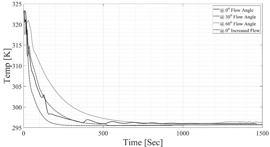
Figure 13. Transient Temperature Profiles
Doubling the velocity at inlet from the constant area will double the volume flow rate. According to first fan law, the RPMs is directly proportional to volume flow rate. In this study volume flow rate is doubled from 0.1 m3 /s to 0.2 m3 /s (i.e. velocity is doubled from 1.3661 m/s to 2.7322 m/s through area 0.0732 m2) keeping other conditions constant and changing the velocity only. So, as per Equation 1, the power consumption by the fan will increase by 8 times.
Conclusion.
Varying the inlet velocity profiles in 2D room, the indoor velocity field and temperature distribution vary significantly as compared to open air. Although by changing velocity, magnitude will produce early and better cooling but more energy will be consumed. By doubling the velocity at inlet, the power consumption will increase 8 times of the initial fan power or the power being consumed just by changing the inlet direction. To achieve similar results without consuming extra energy, change in inlet velocity direction is one of the recommended option. However, change in inlet direction may take little more time than by increasing the velocity only. Steady State temperature of 295.65K is achieved either by doubling the velocity (2.7322 m/s) in 240 seconds or by injecting the air at 30° with 1.3661 m/s in 522 seconds.
Acknowledgement. This manuscript has not been published in other journals previously. This research is supported by CEME, NUST, Pakistan.
Author’s Contribution. Atta ul Mannan Hashmi developed the theory and performed the numerical computations. Arshan Ahmed and Fahad Rafi Butt verified the analytical results. Shahbaz Ghani and Imran Akhtar analyzed effect of various inlet velocity profiles on indoor temperature for energy conservation of HVAC. All authors discussed the results in detail and contributed to the final manuscript.
Conflict of interest. The authors declare no conflict of interest for publishing this manuscript in IJIST.
REFRENCES
[2] K. Horikiri, Y. Yao, and J. Yao, “Numerical simulation of convective airflow in an empty room,” “Int. J. Energy Environ” 2011, vol. 5, no. 1, pp. 574–581.
[3] J. Ni and X. Bai, “A review of air conditioning energy performance in data centers,” “Renew. Sustain. Energy Rev.” 2017, vol. 67, pp. 625–640.
[4] P. Fang, T. Liu, K. Liu, Y. Zhang, and J. Zhao, “A simulation model to calculate temperature distribution of an air-conditioned room,” “Proc. - 2016 8th Int. Conf. Intell. Human-Machine Syst. Cybern. IHMSC” 2016, vol. 1, no. 2, pp. 378–381.
[5] E. Mesenhöller, P. Vennemann, and J. Hussong, “Unsteady room ventilation – A review,” “Build. Environ.” 2020, vol. 169.
[6] A. Raczkowski, Z. Suchorab, and P. Brzyski, “Computational fluid dynamics simulation of thermal comfort in naturally ventilated room,” “MATEC Web Conf.” 2019, vol. 252, p. 04007.
[7] S. Schiavon and A. K. Melikov, “Energy saving and improved comfort by increased air movement,” “Energy Build.” 2008, vol. 40, no. 10, pp. 1954–1960.
[8] M. Wang and Q. Chen, “Assessment of various turbulence models for transitional flows in an enclosed environment (RP-1271),” “HVAC R Res.” 2009, vol. 15, no. 6, pp. 1099–1119.