
Visualizing Impact of Weather on Traffic Congestion Prediction: A Quantitative Study
Shahrukh Hussain1, Usama Munir1, Muhammad Salman Chaudhry1
1Dept. of Computer Science, FCC University Pakistan.
* Correspondence: Muhammad Salman Chaudhry|salmanchaudhry909@gmail.com.
Citation | Hussain. S, Munir. U, Chaudhry. M. S, “Visualizing Impact of Weather on Traffic Congestion Prediction: A Quantitative Study”. International Journal of Innovation in Science and Technology. Vol 3, Special Issue, pp: 210-222, 2022.
Received | Dec 15, 2022; Revised | Feb 17, 2022 Accepted | Feb 18, 2022; Published | Feb 20, 2022.
Abstract.
A substantial amount of research has been done to develop improved Intelligent Transportation Systems (ITS) to alleviate traffic congestion problems. These include methods that incorporate the indirect impact on traffic flow such as weather. In this paper, we studied the impact of weather conditions on traffic congestion along with more spatial and temporal factors, such as weekdays/time and location, which is a different approach to this problem. The proposed solution uses all these indicators to estimate the flow of traffic. We evaluate the level of congestion (LOC) based on the traffic volume grouped in certain regions of the city. The index for the defined LOC indicates the traffic flow from “free -flowing” to “traffic jam”. The data for the traffic volume count is collected from the Department of Transportation (DOT) for NYMTC. Weather conditions along with special and temporal information have an essential role in predicting the congestion level. We used supervised machine learning for this purpose. The prediction models are based on certain factors such as the volume count of the traffic at the entry and exit point of each street pair, particular days of the week, timestamp, geographical location, and weather parameters. The study is done on the major roadways of each of the four prominent boroughs in New York. The results of the traffic prediction model were established by using the Gradient Boosting Regression Tree (GBRT) which showed an accuracy of 97.12%. Moreover, the calculation speed was relatively fast, and it has stronger applicability to the prediction of congestion conditions.
Keywords: Gradient Boosting; Decision Tree Algorithm; Supervised Machine Learning; Traffic Congestion
INTRODUCTION
An enormous increase in urban traffic has been observed recent times, globally [11]. The overall process of modernization is speeding up, leading to the rapid growth of vehicular traffic on roads [12]. To cater the needs for a huge surge in traffic, urban road networks are becoming over complex [13]. Consequently, urban traffic problems are getting serious and traffic congestion is one of them [1]. In metropolitan cities, if the factors leading to the congestion are neglected or, congestion is not predicted and reported properly to the users in time, it can lead the road networks to be paralyzed [14]. The early step to tackle the problem of congestion is to prevent it from happening [14]. Therefore, the establishment of traffic flow, forecasting with respect to the day and time of the day is conducive to the preparation of targeted preventive measures which serve as an early warning [15]. The usage of Intelligent Transportation Systems (ITS) to predict traffic-related information has gained popularity in the field of smart transportation. A well-designed ITS can estimate and inform drivers of the locations and time frame of congested road sections, thus giving them a warning to avoid taking that route [16]. Moreover, it can also provide a significant amount of information for authorities of large metropolitan areas in order to control the parameters of the traffic signal to reduce the Level of Congestion (LOC) [17].
Supervised machine learning models are highly effective and fast with training structured data [18]. However, performance and accuracy of the model is highly dependent upon the dataset since its correct input features and labeling are followed by minimum null values which define accuracy of a model in a real-world [18]. These models are expected to generate adequate results with precision as the datasets become more diverse [19].
In this research paper we have used the supervised machine learning models to estimate the traffic flow and congestion of recent times. The correlations between implicit traffic-related data and weather condition data define influence of values on each other. A detailed exploratory analysis was performed over important weather features that impact congestion on the roads the most, to unveil individual impacts over the traffic flow within the given route at a certain time and day of the week.
The objectives of this research were to examine and evaluate granular relationships between external factors (Weather and ToD (time of day) in our case) with “Traffic Counts” within an area by the use of Supervised Machine Learning Algorithms. The conclusion we reached enabled us to reach a concise evaluation of these 2 factors and paved the way for a future deep-dive into other factors to further quantify an expected traffic count within an area, based on those factors. The objectives were achieved as relationships were established.
BACKGROUND
Researchers from different domains have studied the problem of traffic flow and congestion using various techniques in the past. Statistical analysis is based on a variety of features that lead to the measurement of congestion of vehicles on roads such as motion of the vehicle, stationary time of the vehicle, the velocity of the vehicle, or the cluster of the vehicles within the selected segment of the road network. Data collection is the first step to solve the traffic problems. Various methods including GPS-based [2] and cellular-based [3] sensors installed in smartphones, vehicles, and roadsides, to gather data of geographical location and timestamp. Modern traffic solution are based or safe city cameras and drones etc. to extract the vehicle data from intersections, highways, and freeways. [9] Both the supervised and unsupervised machine learning algorithms have played an integral part in predicting the congestion based on the feature, labeled and unlabeled. In our study, we took the data from each entry and exit of each pair of streets to estimate the traffic congestion and to measure the influence of weather on the overall pattern of traffic flow The main objective of this research is to apply a supervised machine learning model to predict the traffic flow and to examine the impact of weather condition on traffic congestion
RESEARCH QUESTIONS
The following are the research problems that we tackled in our study:
We have used the supervised machine learning model to estimate the traffic flow and congestion in the study. The correlations between implicit traffic-related data and weather conditions, define the influence of values on each other. A detailed exploratory analysis was performed over important weather features that impact congestion on the roads, to unveil individuals’ impacts over the traffic flow within the given route at a certain time and day of the week.
RESEARCH METHODOLOGY
This study utilized various approaches to analyze and use supervised machine learning to produce adequate results with minimal error.
Approach
Supervised machine learning approach has been used in this research to study the problematic statement. With the experiments conducted on the dataset, we were able to make clear judgments, according to the supervised machine learning algorithms for fast and relatively accurate results. All the inputs (features) and outputs are labeled in the dataset which are required to train the model. It is also important to note that the supervised machine learning is mainly used to deal with two problem-sets: classification and regression. For accurate prediction of traffic congestion, the model was trained based on continuous values of the traffic count. Congestion level of traffic count was varied with the help of the classification model. The accuracy and precision of scaled traffic count is used in the research to define the Level of Congestion (LOC).
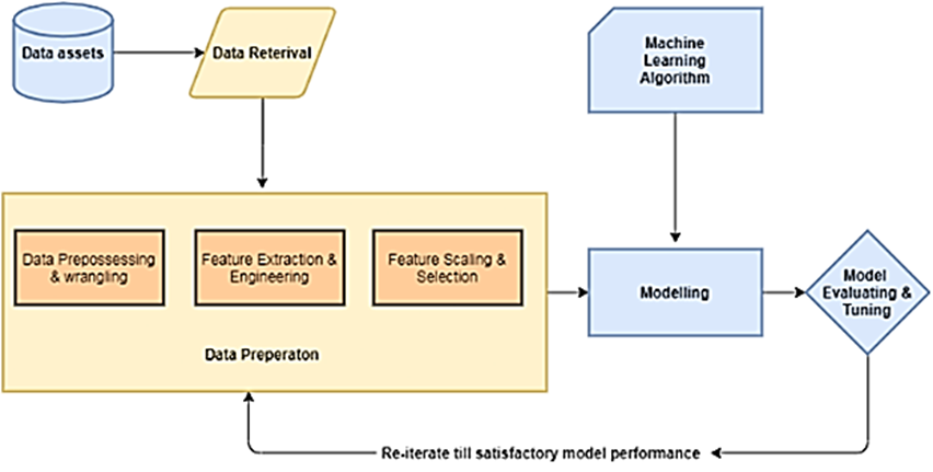
Figure 1. Supervised Machine Learning Pipeline
The basic pipeline can be seen in Figure 1. The workflow for the proposed system in this research diverse involves the ingestion of raw data that has been obtained from source and then applying the data processing techniques to wrangle, processing and engineering meaningful features and attributes from this dataset. All these data preparation steps allow us to train the model which is later used in the testing phase and then for hyper parameter optimization. It helped us in evaluation of a machine learning algorithm that is suitable for the data. The features selected from the data were used in the deployment of the model. The regression- model was used to experiment with the dataset as data comprises of continuous values. The regression model includes independent variables pertaining to month, hour, and a dummy variable for weekends, the geographical clusters variable, and direction, as well as weather data.
Dataset Description
Regarding data acquisition, we took the monthly historical traffic data for the month of March 2018 from the Department of Transportation (DOT) for New York Metropolitan Transportation Council (NYMTC). This data was comprised of its four major Boroughs showing a decent distribution of values found within each Borough with no visible skewness or anomalies observed as stated in .Table 1
Table 1. Borough Distribution
|
No. |
Borough |
Number of Values |
Percentage of Dataset |
|
1 |
The Bronx |
1368 |
27.94% |
|
2 |
Queens |
1152 |
23.53% |
|
3 |
Manhattan |
1320 |
26.96% |
|
4 |
Brooklyn |
1056 |
21.57% |
. The geographical data of 22 streets in boroughs was retrieved using the Google Maps API and acquired the weather data from the external source of same geographical locations and timestamps in our dataset. Weather data acquired of same location had 9 attributes such as cloud cover, precipitation, dew point, relative humidity, precipitation cover, temperature, visibility, conditions, and wind chill.
RESULTS AND DISCUSSION
Exploratory analysis
Various methods and approaches were used for scaling, standardization, and normalization of the dataset for model training and testing to obtain satisfactory outcomes. The parameters comprise of the independent variables – Date, Hourly Time (e.g. 9-10 a.m.), Weather features which further comprise of Conditions, Precipitation, Cloud Cover and Visibility (scaled to obtain a convenient severity level between 0 and 3) to be used for our Regression Model. The dependent variable comprises of the parameter Traffic Count.
Scaling Traffic Count
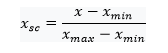
Traffic count, being a continuous value within the data, comprises of values ranging from 0 to 3000 that need to be normalized to a better form to relate it with various features and to extract useful relations with them. For a vigilant representation of co-relations, Traffic Count Label was scaled and grouped by the respective start and end locations. Values were scaled using min-max scalar and scaled into 4 equal divisions from 0 to 3 and termed as Congestion Divisions. The approach behind the min-max scalar is to subtract the minimum value in the feature and then divide it by the range. The range is the difference between the original maximum and original minimum as shown in the Equation 1. The advantage of using a scalar is that the shape of the original distribution is preserved.
Using this min-max scalar, the Level of Congestion (LOC) based on traffic count has been defined and grouped into its respective Borough, which is also normalized. LOC was categorized into 4 discrete values: 0 represents low congestion level, 1 represents mild congestion level, 2 represents slightly high congestion level and finally, 3 represents high congestion level. The distribution of the overall traffic count is shown in the described range from 0 to 3.
Relations with weather features
Based on the domain knowledge, four relevant weather features (Conditions, Precipitation, Cloud Cover, Visibility) were selected that could influence the traffic count. Values were scaled to obtain a convenient severity level between 0 and 3, . The scaled divisions were made, based on domain knowledge related to that feature. Finally, values were compared with Scaled Traffic count to observe the strongest intersection of similar severity values to depict influence. The greater the number of overlapping of similar severities, the greater will be the influence.
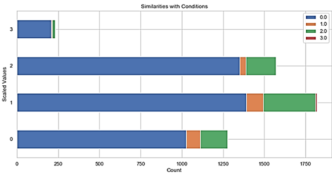
Figure 2. Relation Count Distribution of Conditions and Scaled Count.
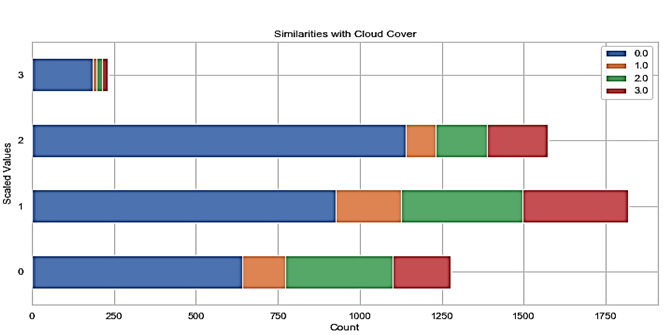
Figure 3. Relation Count Distribution of Cloud Cover and Scaled Count.
Comparison of scaled severity values of weather features with Traffic Count showed that greatest intersections arose with Conditions and Cloud Cover as shown in Figure 2. And Figure 3. Further evaluation was made in the Feature Analysis section.
Relations with Time of Day
Peak times were to be analyzed from the entire dataset i.e., all given locations to depict where the greatest traffic count was observed in case of a Weekday and a Weekend, to evaluate the importance of ‘Type of Day’.
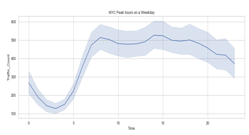
Figure 4. Peak hours on a Weekday
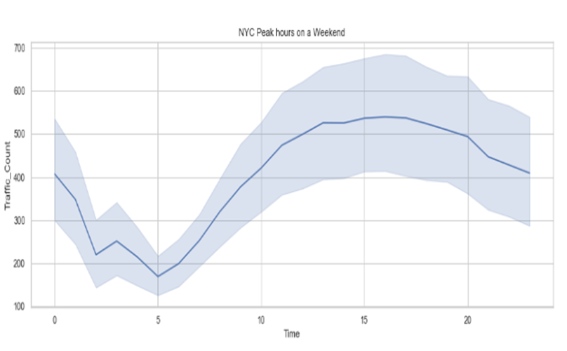
Figure 5. Peak hours on a Weekend
According to both figures, the peak hour ranges showed distinguishable variations on both Weekdays and Weekends. On a weekday, the peaks were found to be on 2-3 pm and 8-9 pm and for the weekends, these were found to be between 2-7 pm, indicating greater peak hours and traffic counts on Weekends.
MODEL SELECTION
Base Accuracy
Since our target label i.e., Traffic count was observed continuous in nature, Regression Model was implemented as a means to provide the best coordination. Tested models comprised of Linear Regression, Lasso Regression, Decision Trees, Random Forest Regression (RF) [6], and Gradient Boosting Regression Tree (GBRT). Among all, Random Forest showed the best results with an accuracy of 96.14%.
Actual VS Predicted
The accuracy Score of all the models was validated by relating their predicted values with the original targeted values by plotting them against each other and subsequently, visualizing the integrated result. The minimum difference in values i.e., which were found on densely populated sites closer to the baseline was considered as possessing least error, while the ones distant from them can be termed as anomalies as shown in Figure 6.
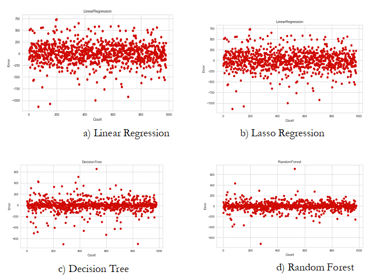
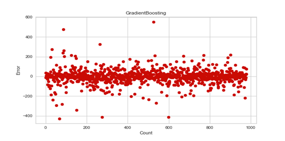
e) Gradient Boosting Regression Tree
Figure 6. Model Accuracy VS Precision. Number of data values represented on x-axis and error on y-axis. Plotted coordinates represent the difference between actual and predicted values with density of points near base indicating greater accuracy.
Hyper parameter Optimization
After optimizing the hyper-parameters of all the regression models selected for this research, it was observed that the base accuracy of the Gradient Boosting Regression Tree was increased from 92.39% to 97.12% using the Grid Search CV and validation of the model was evaluated by the shuffle spilt validation. Overall, we observed an improvement of 5.12% in the model accuracy. The gradual increment can be observed in Table 2.
Table 2. Parameter-Tuning Accuracy
|
Accuracy |
n-estimators |
Max-depth |
Min-sample-leaf |
Max-sample-split |
|
92.39% |
100 |
3 |
1 |
2 |
|
94.38% |
200 |
3 |
1 |
2 |
|
95.90% |
100 |
5 |
1 |
2 |
|
92.83% |
100 |
3 |
2 |
2 |
|
92.83% |
100 |
3 |
1 |
5 |
|
96.22% |
200 |
5 |
2 |
5 |
|
96.42% |
400 |
5 |
2 |
5 |
|
96.62% |
400 |
7 |
2 |
5 |
|
97.12% |
400 |
7 |
5 |
5 |
|
96.67% |
600 |
7 |
5 |
10 |
MODEL EVALUATION
Although after rigorous experimentation with optimized hyper-parameters of the selected models, the correct validation results were generated to evaluate the performance of the model on training data. However, the fit of a proposed regression-based model should therefore be better than the fit of the mean model, so all models were evaluated via R2 error in which the ratio of the variance of the model and the total variance of target variable was taken and put forward a value between 0 and 1 with 1 being the best one. MAE was also used to identify the difference between the forecasted value and the actual value. The general definition of the R2 score can be seen in Equation 2.

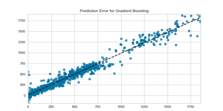
Figure 7.R2 Accuracy for Gradient Boosting
Feature analysis
Trained model was tested for co-relations among all the existing features which showed vibrant relations of Traffic Count with weather as standing out among all other weather features with the greatest feature importance, also observed in Figure 5, similar to our prior exploratory analysis in the section.
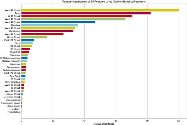
Figure 8. Feature Importance
Discussion
On successfully recording, the highest accuracy of our model GBRT, the predicted results were visualized via a heat map through the Folium library. The visualized points indicated the coordinates of the start and end of the street locations of the designated routes within the data. Furthermore, the intensity of the color of the marker of that location expresses the intensity of traffic flow in that particular route. It ranges into 4 severity levels of congestion with a color palette of blue, green, and yellow. The red color indicates a relatively high traffic flow and a darker blue color represents a relatively low traffic flow. Visualized results for a time duration of 7:00-8:00 am describe the peak hour for the traffic flow, leading to congestion, as seen in the Figure 6. With the help of the visualization, the traffic pattern can be studied and understood.
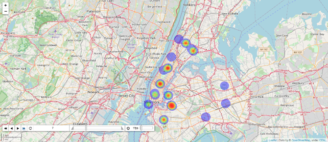
Figure 9. Visualized Results
CONCLUSION AND FUTURE SCOPE
After detailed analysis, the conclusion can be made that external factors like weather (in our case) do impact traffic congestion as a whole for the given dataset and that our Gradient Boosting Regression Tree model records the best accuracy score for predicting Traffic Count parameters i.e. 97.12% considering all relevant features as mentioned in Table 3. On the contrary, the greatest feature importance examined among all the weather features was Weather Conditions, followed by Wind Chill.
Table 3. Model Accuracy
|
Model |
Base Accuracy |
After Hyper parameter Tuning |
|
Linear Regression |
75.23% |
71.60% |
|
Lasso Regression |
75.22% |
71.50% |
|
Decision Tree |
93.24% |
94.10% |
|
Random Forest |
96.14% |
96.80% |
|
Gradient Boosting |
92.39% |
97.12% |
In this paper, the model is based on regular day predictions. However, we look forward to the implementation of a more robust model that will also consider the Planned Special Events (PSEs), like festival holidays, social events like concerts, sporting events like cricket and football matches and so on. Moreover, seasonal changes may also affect the traffic flow adversely because of the ambiguities in weather they may bring. Therefore, we also look forward to work with this aspect. We believe our research will pave the way for greater opportunities in the field of data gathering and will help in developing a more stabilized road network of the city that is less prompted to traffic congestion.
Conflict of interest. The Authors have no conflict of interests.
Project details. Nil.
REFERENCES
[1] Sweet, M. “Traffic Congestion’s Economic Impacts: Evidence from US Metropolitan Regions”. 2013 SAGE journals-Urban Studies, vol. 51, pp. 2088-2110, 2013
[2] Thianniwet, Thammasak & Phosaard, Satidchoke & Pattara-atikom, Wasan. “Classification of Road Traffic Congestion Levels from GPS Data using a Decision Tree Algorithm and Sliding Windows”. 2009 World Congress on Engineering, vol. 1, 2009
[3] Jahangiri, A., &Rakha, H. A. “Applying Machine Learning Techniques to Transportation Mode Recognition Using Mobile Phone Sensor Data”. IEEE Transactions on Intelligent Transportation Systems, vol. 16, pp. 2406–2417, 2018
[4] Jayapal, C., & Roy, S. S. “Road traffic congestion management using VANET”, 2016 International Conference on Advances in Human Machine Interaction (HMI), 2016
[5] P. Chhatpar, N. Doolani, S. Shahani, and R. Priya, “Machine learning solutions to vehicular traffic congestion,” 2018 International Conference on Smart City and Emerging Technology (ICSCET), 2018.
[6] Y. Liu and H. Wu, “Prediction of road traffic congestion based on random forest,” 2017 10th International Symposium on Computational Intelligence and Design (ISCID), vol. 2, 2017
[7] Chowdhury, B.,Kinhikar, M. &Alleema, N. N. “Road Traffic Prediction using Machine Learning”. International Research Journal of Engineering and Technology (IRJET). Vol. 06, 2019
[8] M. M. Chowdhury, M. Hasan, S. Safait, D. Chaki, and J. Uddin, “A traffic congestion forecasting model using cmtf and machine learning,” 2018 Joint 7th International Conference on Informatics Electronics and Vision (ICIEV) and 2018 2nd International Conference on Imaging, Vision and Pattern Recognition (icIVPR), 2018
[9] Huang, F.-R., Wang, C.-X., & Chao, C.-M. “Traffic Congestion Level Prediction Based on Recurrent Neural Networks”. 2020 International Conference on Artificial Intelligence in Information and Communication (ICAIIC), 2020
[10] Jia Lu, & Li Cao. “Congestion evaluation from traffic flow information based on fuzzy logic”. 2003 IEEE International Conference on Intelligent Transportation Systems., 2003
[11] Sun Ye. “Research on Urban Road Traffic Congestion Charging Based on Sustainable Development”. International Conference on Applied Physics and Industrial Engineering, Physics Procedia 24 pp. 1567–1572, 2012
[12] Ge Shi, Jie Shan, Liang Ding, Peng Ye, Yang Li, Nan Jiang. “Urban Road Network Expansion and Its Driving Variables: A Case Study of Nanjing City”. International Journal of Environmental Research and Public Health, 16, pp. 2318, 2019
[13] Gao ZH, Chen ZJ, Liu YX, Huang K (2007) Study on the complex network characteristics of urban road system based on GIS. Proceedings of SPIE 6754:67540N
[14] S R Samal1, P Gireesh Kumar2, J Cyril Santhosh3, and M Santhakumar. “Analysis of Traffic Congestion Impacts of Urban Road Network under Indian Condition”. IOP Conf. Series: Materials Science and Engineering, 2020
[15] Z. Yin, J. Wang and H. Lu, “A Study on Urban Traffic Congestion Dynamic Predict Method Based on Advanced Fuzzy Clustering Model,” 2008 International Conference on Computational Intelligence and Security, 2008, pp. 96-100, doi: 10.1109/CIS.2008.194.
[16] Jarašūnienė, Aldona. (2007). Research into Intelligent Transport Systems (ITS) technologies and efficiency. TRANSPORT. 22. 61-67, 2010
[17] Wei-Hsun Lee and Chi-Yi Chiu. “Design and Implementation of a Smart Traffic Signal Control System for Smart City Applications”. Sensors 2020, 20, 508; doi:10.3390/s20020508
[18] Sarker, I.H. Machine Learning: Algorithms, Real-World Applications and Research Directions. SN COMPUT. SCI. 2, 160 (2021). https://doi.org/10.1007/s42979-021-00592-x
[19] Abdulraheem, Ajiboye & Abdullah Arshah, Ruzaini & Qin, Hongwu. (2015). Evaluating the Effect of Dataset Size on Predictive Model Using Supervised Learning Technique. International Journal of Software Engineering & Computer Sciences (IJSECS). 1. 75-84. 10.15282/ijsecs.1.2015.6.0006.